Timing Code and Simple Speed-up Techniques
Overview
Teaching: 30 min
Exercises: 45 minQuestions
How can I time my code
What is the difference between vectorisation and for loops?
What is the cache?
How can
lru_cachespeed up my code?Objectives
Introduce
time,timeitmodules for timing code andcProfile,pstatsfor code profiling
![]()
Performance Measurement
Before diving into methods to speed up a code, we need to look at some tools which can help us understand how long our code actually takes to run. This is the most fundamental tool and one of the most important processes that one has to go through as a programmer.
Performance code profiling is a tool used to identify and analyse the execution of applications, and identify the segments of code that can be improved to achieve a better speed of the calculations or a better flow of information and memory usage.
This form of dynamic program analysis can provide information on several aspects of program optimization, such as:
- how long a method/routine takes to execute
- how often a routine is called
- how memory allocations and garbage collections are tracked
- how often web services are called
It is important to never try and optimise your code on the first try. Get the code correct first. It is often said that premature optimization is the root of all evil when it comes to programming.
Before optimising a code, one needs to find out where the time is spent most. Around 90% of the time is spent in 10% of the application.
There are a number of different methods and modules one can use
timetimeitcProfiledatetimeastropy- mainly for astronomy usage- Full fledged profiling tools: TAU, Intel Vtune, Python Tools for Visual Studio, etc.
time module
Python’s time module can be used for measuring time spent in specific part of the program. It can give the absolute
real-world time measured from a fixed point in the past using time.time(). Additionally, time.perf_counter() and
time.process_time() can be used to derive the relative time. unit-less value which is proportional to the time
elapsed between two instants.
import time

print (time.time())

print (time.perf_counter()) # includes time elapsed during sleep (CPU counter)
print (time.process_time()) # does not include time elapsed during sleep
1652264171.399796
2.433484803
0.885057
It’s main use though is to take the time.time() function and assign it to a variable, then have the function which
you want to time, followed by a second call of the time.time() function and assign it to the new variable. A quick
arithmetic operation will quickly deduce the length of time taken for a specific function to run.
t0 = time.time()

my_list = []
for i in range(500):
    my_list.append(0)

t1 = time.time()

tf = t1-t0

print('Time taken in for loop: ', tf)
Time taken in for loop: 0.00011992454528808594
timeit module
This can be particularly useful as it can work in both python files and most importantly in the command line interface.
Although it can be used in both, it’s use is excellent in the command line. The timeit module provides easy timing
for small bits of Python code, whilst also avoiding the common pitfalls in measuring execution times. The syntax from
the command line is as follows:
$ python -m timeit -s "from my module import func" "func()"
10 loops, best of 3: 433 msec per loop
In a Python interface such as iPython, one can use magics (%).
In [1]: from mymodule import func
In [2]: %timeit func()
10 loops, best of 3: 433 msec per loop
Let us look at an example using the Montecarlo technique to estimate the value of pi.
import random as rnd
import math


def montecarlo_py(n):
    x, y = [], []
    for i in range(n):
        x.append(rnd.random())
        y.append(rnd.random())
    pi_xy = [(x[i], y[i]) for i in range(n) if math.sqrt(x[i] ** 2 + y[i] ** 2) <= 1]
    return(4 * len(pi_xy) / len(x))
    # Estimate for pi
Our modules math, random are imported for the calculation, and the function returns an estimate for pi given n
number of points. Running the program can be done as so, and will produce a result close to 3.14.
montecarlo_py(1000000)
If we want to time this using timeit we can modify the above statement using cell magics, and it will not produce the
result, but rather the average duration.
%timeit montecarlo_py(1000000)
724 ms ± 6.52 ms per loop (mean ± std. dev. of 7 runs, 1 loop each)
You can implement a more controlled setup, where one sets the number of iterations, repetitions, etc, subject to the use case.
import timeit

setup_code = "from __main__ import montecarlo_py"
stmt = "montecarlo_py(1000000)"
times = timeit.repeat(setup=setup_code, stmt=stmt, repeat=3, number=10)
print(f"Minimum execution time: {min(times)}")
Minimum execution time: 7.153229266
cProfile
cProfile provides an API for profiling your Python program. A profile is a set of stats showing the time spent in
different parts of the program. In bash you can use a profile statement to save results to a file func.prof.
cProfile.run('func()', 'func.prof')
Alternatively, you can call it in Python.
import cProfile
cProfile.run('montecarlo_py(1000000)')
         5000007 function calls in 1.391 seconds

   Ordered by: standard name

   ncalls  tottime  percall  cumtime  percall filename:lineno(function)
        1    0.495    0.495    0.558    0.558 <ipython-input-3-7987cc796f5a>:11(<listcomp>)
        1    0.501    0.501    1.338    1.338 <ipython-input-3-7987cc796f5a>:6(montecarlo_py)
        1    0.053    0.053    1.391    1.391 <string>:1(<module>)
        1    0.000    0.000    1.391    1.391 {built-in method builtins.exec}
        2    0.000    0.000    0.000    0.000 {built-in method builtins.len}
  1000000    0.063    0.000    0.063    0.000 {built-in method math.sqrt}
  2000000    0.128    0.000    0.128    0.000 {method 'append' of 'list' objects}
        1    0.000    0.000    0.000    0.000 {method 'disable' of '_lsprof.Profiler' objects}
  2000000    0.150    0.000    0.150    0.000 {method 'random' of '_random.Random' objects}
This can be modified to save the output to a .prof file.
cProfile.run('func()', 'func.prof')
But there is not much point of this for a small function like this which has a limited runtime. We will look at another
file, and this time run it through the terminal, and generate the .prof file.
python -m cProfile -o heat_equation_simple.prof heat_equation_simple.py
Running Time: 20.20987105369568
It’s all well and good creating a .prof file, but we need a separate module to look at the profile we have just
created.
Investigating profiles with pstats
This is step 2 in profiling, analysing the profile and seeing where our functions are experiencing bottlenecks.
pstats prints execution time of selected functions, while sorting by function name, time, cumulative time, etc. It is
a python module interface and has an interactive browser.
from pstats import Stats
p = Stats('heat_equation_simple.prof')

p.strip_dirs() #The strip_dirs() method removes the extraneous path from all the module names

# Other string options include 'cumulative', 'name', 'ncalls'
p.sort_stats('time').print_stats(10)
Day Month Date HH:MM:SS Year    heat_equation_simple.prof

         1007265 function calls (988402 primitive calls) in 22.701 seconds

   Ordered by: internal time
   List reduced from 5896 to 10 due to restriction <10>

   ncalls  tottime  percall  cumtime  percall filename:lineno(function)
      200   20.209    0.101   20.209    0.101 evolve.py:1(evolve)
      797    0.841    0.001    0.841    0.001 {built-in method io.open_code}
    68/66    0.178    0.003    0.183    0.003 {built-in method _imp.create_dynamic}
        1    0.135    0.135    0.135    0.135 {built-in method mkl._py_mkl_service.get_version}
      797    0.128    0.000    0.128    0.000 {built-in method marshal.loads}
      797    0.118    0.000    0.118    0.000 {method 'read' of '_io.BufferedReader' objects}
     3692    0.059    0.000    0.059    0.000 {built-in method posix.stat}
      797    0.043    0.000    1.002    0.001 <frozen importlib._bootstrap_external>:969(get_data)
 2528/979    0.038    0.000    1.107    0.001 {built-in method builtins.__build_class__}
       36    0.035    0.001    0.035    0.001 {built-in method io.open}
Using this for longer programs and more functions can help you pin down the functions in your code which need optimisation. Using pstats in the terminal is fairly simple, as it is incorporated into the python command. We will get a chance to try this out shortly.
$ python -m pstats myprof.prof
Welcome to the profile statistics
% strip
% sort time
% stats 5

Day Month Date HH:MM:SS Year my.prof
...
Montecarlo Pi
There are three functions in the code block below. Each is a slightly different implementation of a Montecarlo algorithm for calculating the value of pi. Use
time.time(),%timeit,cProfileandpstatsto learn how the functions work. Are the timings what you would expect? What implementation is fastest for 1 million points?
pi_estimation_pure()is a pure Python implementation using lists.
pi_estimation_loop()uses numpy arrays to replace the python lists.`pi_estimation_np() uses numpy to improve the performance of the algorithm.
Hint: You may want to try writing the three functions to a file and running
cProfileon that file. You can use the ipython magic%%writefileif you are using a notebook.import math import random as rnd import numpy as np import time def pi_estimation_pure(n): # TODO x, y = [], [] for i in range(n): x.append(rnd.random()) y.append(rnd.random()) pi_xy = [(x[i], y[i]) for i in range(n) if math.sqrt(x[i] ** 2 + y[i] ** 2) <= 1] # TODO # return 4 * len(pi_xy) / len(x) def pi_estimation_loop(n): count=0 # TODO for step in range(n): x=np.random.rand(1) y=np.random.rand(1) if math.sqrt(x*x+y*y)<1: count+=1 # TODO # return 4*count/n def pi_estimation_np(n): # TODO p=np.random.rand(n,2) p_est = 4*np.sum(np.sqrt(p[:,0]*p[:,0]+p[:,1]*p[:,1])<1)/n # TODO # return p_estYou can check the execution times using the following:
pi_estimation_pure(1000000)
pi_estimation_loop(1000000)
pi_estimation_np(1000000)
Solution
You can find the solution in the notebook.
Profiling the heat equation
The file
heat_equation_simple.pycontains an inefficient implementation of the two dimensional heat equation. UsecProfileandpstatsto find where the time is most spent in the program.Compare with the file
heat_equation_index.pya more efficient version that uses indexing rather than for loops.
NumPy - Fast Array Interface
Python lists
Python lists are one of the 4 main data types in Python:
- lists
[1,2,3] - tuples
(1,2,3) - dictionaries
{"Food" : "fruit", "Type" : "banana"} - sets
{"apple", "banana"}

Lists are ordered, changeable, start at index [0], and can store all types of variables, including other data types.
# Flexiblilty of standard python array
a = [1, 2.1, '3', (4, 5.2), [6, {7.3 : '8'}, 9]]
a
[1, 2.1, '3', (4, 5.2), [6, {7.3: '8'}, 9]]
Python lists have the following features
- Dynamic, elements of different types, including other types of ‘array’
- Multiple dimensions
- Subarrays can have different number of elements
In short they are very flexible but not good in practice, why?
- Python has the luxury of being programmable without the user caring about the data types they are using.
- Lists may be flexible but also slow to process in numerical computations.
- These are arrays of pointers to objects in sparse locations in memory, which cannot be easily cached and thus reading its values becomes a slower task.
To become efficient in data-driven programming and computation requires a good understanding of how data is stored and manipulated. This will help you in the long run. In statically typed languages like C++ or Java, all the variables have to be declared explicitly, a dynamically typed language like Python skips this step and is why it is more popular. This does have drawbacks when it comes to performance.
Thankfully, simple libraries like NumPy can assist with this.
NumPy arrays
NumPy arrays are a massive upgrade to the Python lists. There are some slight disadvantages, but in all, the advantages for outweigh the disadvantages.
- Provides a convenient interface for working with multi-dimensional array data structures efficiently.
- Arrays use contiguous blocks of memory that can be effectively cached by the CPU.
- NumPy sacrifices Python’s flexibility to achieve low-memory usage and speed-up, as NumPy arrays have a fixed size and the datatype of its element must be homogeneous.
- Written in C, which is known for being a efficient programming language in terms of speed and memory usage.
NumPy arrays can be created from a Python list or tuple by using NumPy’s array function. The dimensionality and shape of the resulting array will be determined by the given input. NumPy offers several functions for creating arrays, depending on the desired content and shape of the array.
When creating an array, NumPy will try to convert entries to convenient data type. If it is not possible, it will raise
an error. Feel free to check out the link to Numpy documentation for more information.
array
import numpy as np
# Creation from Python list
a = np.array((1,'2',3,4), float)

# Creation of 3D numpy array
b = np.array([[[1, 2.2],[3, 4]],[[5,6.6],[7.8, 9]]])

print("a: NumPy array from Python list\n", a, "\n")
print("b: 3D NumPy array\n", b)
a: NumPy array from Python list
 [1. 2. 3. 4.]

b: 3D NumPy array
 [[[1.  2.2]
  [3.  4. ]]

 [[5.  6.6]
  [7.8 9. ]]]
The main features of the above NumPy array are:
- It has multiple dimensions
- All elements have the same type
- Number of elements in the array is fixed
Understanding the shape and size of arrays is crucial in applications such as machine learning and deep learning. You will often need to reshape arrays.
# Determine shape of array b
print("Array b:\n", b,)
print("\nShape:\n", b.shape)
print("\nSize:\n", b.size, "\n")

# Reshape b into a 1x8 matrix
b_new = b.reshape(1,8)
print("Array b_new:\n", b_new, b_new.shape, b_new.size)
Array b:
 [[[1.  2.2]
  [3.  4. ]]

 [[5.  6.6]
  [7.8 9. ]]]

Shape:
 (2, 2, 2)

Size:
 8

Array b_new:
 [[1.  2.2 3.  4.  5.  6.6 7.8 9. ]] (1, 8) 8
This is fine, but creates an issue with storage, particularly for large arrays. As we no longer need array b, we can
get rid of it using del.
del b
print(b)
---------------------------------------------------------------------------
NameError                                 Traceback (most recent call last)
<ipython-input-14-67e500defa1b> in <module>
----> 1 print(b)

NameError: name 'b' is not defined
In statically typed languages, one should always free up the memory taken up by variables, usually with keywords such as
free in C.
NumPy Array Indexing
Indexing and Slicing are the most important concepts in working with arrays. We will start with indexing, which is the
ability to point and get at a data element within an array. Indexing in Python, and most programming languages starts
at the value of 0. The first element of the array is index = 0, the second has index = 1 and so on. Let’s see how
we can use indexing to index the elements of a 1D, 2D and 3D array.
mat1d = np.array([1,2,3,4,5,6])
print(mat1d[1])

mat2d = np.array([[1,2,3], [4,5,6]])
print(mat2d[0,2], mat2d[:1])

mat3d = np.random.randint(1,50,(4,2,4))
print(mat3d)
print(mat3d[3,1,2])
2

3 [[1 2 3]]

[[[ 1 14 31 28]
  [ 2 32 38 33]]

 [[22 29 35  5]
  [47 38 10 37]]

 [[44  7 49 34]
  [ 7 15  2 45]]

 [[15 27 37 11]
  [38 40 34  7]]]

34
Slicing is also an important feature. Say that you have a very large array, but you only want to access the first n
elements of the array, you would use slicing to do so. You call your array, then in square brackets tell it the start
and end index that you want to slice.
In the example of the first n elements of an array called my_array, the notation would be my_array[0:n-1]. There
are more examples below.
mat1d = np.arange(10)
print(mat1d)
mat1d[3:]
[0 1 2 3 4 5 6 7 8 9]
array([3, 4, 5, 6, 7, 8, 9])
You can also slice using negative indexes, and call using steps. Say in an array of 0 to 100 you only wanted to grab the even or odd numbers.
print(mat1d[:-2])

print(mat1d[1:7:2])

mat3d = np.random.randint(1,10,(4,3,4))
print(mat3d)
array([0, 1, 2, 3, 4, 5, 6, 7])

array([1, 3, 5])

[[[7 1 6 6]
  [5 5 9 2]
  [2 1 3 3]]

 [[4 6 7 3]
  [3 5 1 3]
  [2 5 2 9]]

 [[7 2 5 3]
  [9 3 7 9]
  [9 1 2 4]]

 [[7 1 4 4]
  [3 5 9 4]
  [5 3 7 9]]]
mat3d[0:3, 0:2, 0:4:2] = 99
mat3d
array([[[99,  1, 99,  6],
        [99,  5, 99,  2],
        [ 2,  1,  3,  3]],

       [[99,  6, 99,  3],
        [99,  5, 99,  3],
        [ 2,  5,  2,  9]],

       [[99,  2, 99,  3],
        [99,  3, 99,  9],
        [ 9,  1,  2,  4]],

       [[ 7,  1,  4,  4],
        [ 3,  5,  9,  4],
        [ 5,  3,  7,  9]]])
There are many possible ways of arranging items of an N-dimensional array in a 1-dimensional block. NumPy uses striding
where N-dimensional index; n_0, n_1, ... n_(N-1) corresponds to offset from the beginning of 1-dimensional block.
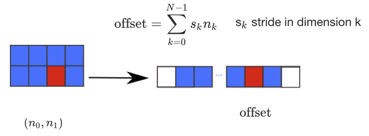
a = np.array(..)
a.flags- Various information about memory layout.a.strides- Bytes to step in each dimension when traversing.a.itemsize- Size of one array element in bytes.a.data- Python buffer object pointing to start of arrays data.a.__array_interface__- Python internal interface.
This should be familiar, so feel free to check out the NumPy documentation for more utilisation of functions.
Vetorisation
We should all be familiar with for loops in Python, and its reputation. Ideally we should be using vectorisation, which begs the question… why?
- for loops in Python are very slow
- vectorisation is an example of a SIMD operation
- one instruction carries out many operands in parallel
- less overhead compared to for loops
Lets look at a difference example:
def loop_it(n):
    t0 = time.time()
    arr = np.arange(n)
    dif = np.zeros(n-1, int)
    for i in range(1, len(arr)):
        dif[i-1] = arr[i] - arr[i-1]
    t1 = time.time()
    print('Loop version: {} seconds'.format(t1-t0))
    return dif

def vectorise_it(n):
    t0 = time.time()
    arr = np.arange(n)
    dif = arr[1:] - arr[:-1]
    t1 = time.time()
    print('Vectorised version: {} seconds'.format(t1-t0))
    return dif

n=10000000
loop_it(n)
vectorise_it(n)
Loop version: 4.1977081298828125 seconds
Vectorised version: 0.02220916748046875 seconds
array([1, 1, 1, ..., 1, 1, 1])
Arrays, slicing and powers array
Head to the Jupyter notebook and do the NumPy exercises.
Solution
Head to the solutions notebook.
Caching
You may ask… what is the cache? The cache is a part of the computer’s memory. Caching can provide an application performance boost as it is faster to access data from the temporary location than it is to fetch the data from the source each time. A computer’s memory can consists of three elements
- Main memory (RAM or ROM):
- Secondary memory
- Cache: Acts as a buffer betwwen the CPU and main memory, used to hold parts of data and program most frequently used by the CPU.
There are a few main rules of caching:
- If a function is frequently called, its output is not changing often and it takes a long time to execute, it is a suitable candidate to implement caching.
- Caching should be faster than getting the data from the current data source
- Caching impacts memory footprint, so it is crucial to choose and cache the data structures and attributes that need to be cached.
Caching itself is an optimization strategy that you can use in your applications to keep recent or often used data in memory locations that are faster to access.
The LRU (Least Recently Used) Cache discards the least recently used items first. The algorithm keeps track of what was used. The functools module deals with high-order functions, specifically:
- functions which operate on other functions
- returning functions
- other callable objects
The lru_cache() helps reduce the execution time of the function by using the memoization technique.
Let’s have a look at caching in action for the Fibonacci sequence. The least recently used algorithm can cache the return values that are dependent on the arguments that have been passed to the function.
def fib(n):
    if n < 2:
        return n
    else:
        return fib(n-1) + fib(n-2)

t1 = timeit.Timer("fib(40)", "from __main__ import fib")

print(t1.timeit(1))
27.941036257019732
from functools import lru_cache

@lru_cache(maxsize=100)
def fib(n):
    if n < 2:
        return n
    else:
        return fib(n-1) + fib(n-2)

t1 = timeit.Timer("fib(40)", "from __main__ import fib")

print(t1.timeit(1))
7.97460088506341e-05
Climbing stairs
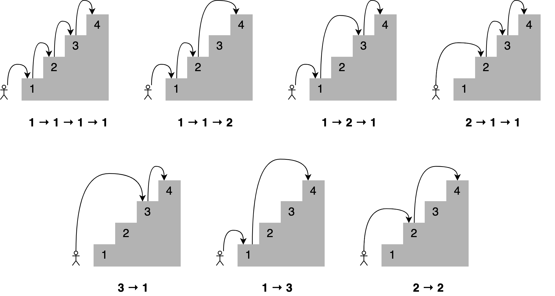
Imagine you want to determine all the different ways you can reach a specific stair in a staircase by hopping one, two, or three stairs at a time.
How many paths are there to the fourth stair? Here are all the different combinations.
A solution to this problem is to state that;
To reach your current stair, you can jump from one stair, two stairs, or three stairs below.</b>
Adding up the number of jump combinations you can use to get to each of those points should give you the total number of possible ways to reach your current position.
For 4 stairs, there are 7 combinations. For 3 there is 4, and for 2 there is 2.
The file
stairs.pyimplements recursion to solve the problem.Create a timing setup and record the time taken for 40 iterations. Then implement the lru_cache and compare the improvement.
Solution
You can find the solution in the Jupyter notebook.
Key Points
Performance code profiling is used to identify and analyse the execution and improvement of applications.
Never try and optimise your code on the first try. Get the code correct first.
Most often, about 90% of the code time is spent in 10% of the application.
The
lru_cache()helps reduce the execution time of the function by using the memoization technique, discarding least recently used items first.