Python in HPC
Overview
Teaching: 15 min
Exercises: 5 minQuestions
Why would one use Python in High Performance Computing?
What is Python’s reference counter and garbage collector?
What are the different parallelisation strategies for Python?
Objectives
Log into ICHEC’s cluster and Jupyterhub
How to import images, code snippets and abstractions
How to structure callouts, highlighting
![]()
Python and its applicability in HPC
Many of you, when you think of Python, think of the snake, but the origin of the name Python actually comes from the very popular Monty Python series, starring John Cleese, Michael Palin and so on which was broadcasted in the 70s as a skit comedy show. It is also highly recommended viewing! The creators of the language really enjoyed the show, and they named it after the show rather than the snake.
It is a high level objective oriented language as I am sure many of you know and ideal for rapid development. But if you have an easy to use language, one that has simple syntax, has a thriving community and is versatile.
When one thinks of high performance computing, python shouldn’t really be in the same sentence. Why? Because python, by the way that the language actually works and is constructed.
Why do we use Python though? In short…
- It’s simple
- Fully featured with basic data types, modules, error handling
- Easy to read
- Extensible in C, C++, Fortran
- Has a large community, third party libraries, tools
- Portable and free
This is all well and good, and working with Python is often a go to for day to day programmers. So what is the problem? Shouldn’t Python be the obvious choice for working on an HPC?
You probably have guessed why, especially if you have been working with Python for a few months. It’s slow!
All the above points as to why Python is such a great language to use does unfortunately impact on its performance. Although Python is itself written in C under the hood, its dynamic nature and versatility causes it to be a poor performer compared to other languages such as C and Fortran.
This course however, with the use of correct use of language, and reworking your code with other external libraries can really assist in speeding up your code and more importantly, use it at scale.
First though, we will make sure you can log into ICHEC systems.
Logging in
Often one of the more complex items on the agenda is effectively logging in. We recommend having two terminal windows open for this. You have been given a course account in the form
courseXXover the last few days, which you will need to log in. If you are already an ICHEC user and are partaking in this course live, please use your course account only.You can log in using the following command;
$ ssh courseXX@kay.ichec.ieFrom here you will need the password for your ssh key (if you made one) followed by the course account password which will have been provided to you by your instructor. Once logged in we will then go into logging into ICHEC’s JupyterHub!
Python’s reference counting and garbage collector
Let us move onto reference counting and garbage collection. This is a very high level overview of the memory management in Python. It is more complicated in reality, but this will give an overview to have a good idea of the governing principles.
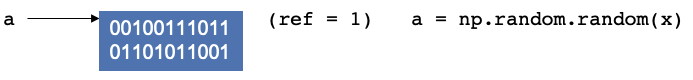
Let’s consider the example where a script that starts by creating a random numpy array and assigning it to a variable
a. In the background, you are creating a location in memory, that is continuous with some binary notation inside it.
When you create somethin, Python will update the reference count. The reference refers to the number of variables that
point to the allotted location in memory. The reference is not to the variable, but to the location. If you have worked
with C, C++ this concept should be fairly familiar.

Now let’s create another operation and continue in the script, say you create a transpose of a and assign it to b,
it doesn’t create new memory. Instead, the operation does some changes and reuses the same block of memory, as it is
used by two variables, and the reference counter will increase by 1.
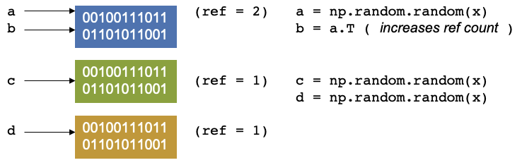
Let us continue our script again. We create have two other arrays, c and d, let us keep them the same size, our
reference counters will be 1 and 1.
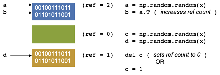
Now let us say we delete c, Our reference counter decreases as there is no variables that point to that block of
memory. The memory location has no variable pointing to it. There is another concept called garbage collection which
are cycles that occur in Python. It is a mechanism that checks through the memory and when it finds that a memory
location has a reference equal to 0, then the garbage collector will mark it as free. But the memory appears as free to
Python, but not to anything outside of Python. You effecitvely see it as a black box and so does the operating system.
Python however, sees it as an empty black box it can use. If you create a new variable, it may put it into this space
in memory. You can also reduce the reference count by setting c = 1, so that it now points somewhere else.
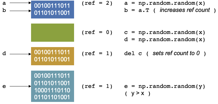
Continuing with our script, if we allocate an array, e of size = y, where y > x, then the memory doesn’t fit, and
unlike a gas being able to become pressurised as it fits into a small container, we cannot fit this in in the same way
as we cannot fit a litre of water in a teacup.
The memory of NumPy arrays is allocated as a continuous block only. So the block will be unused and will only be used if you create something later that fits in the memory. If that happens Python can allocate the memory, reuse it and set the reference counter to 1 again.
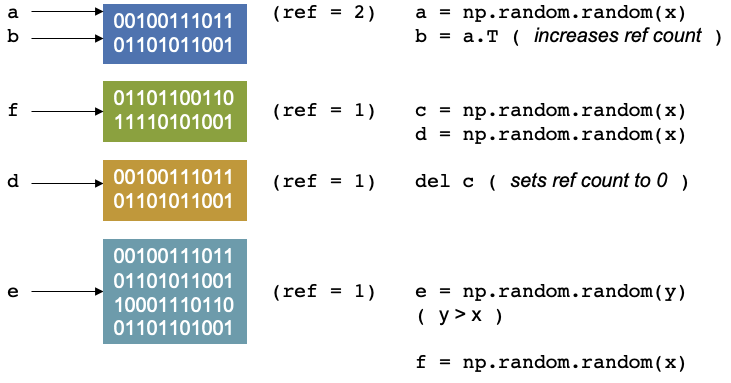
It will only be used up if you create a new item (which we will call f) which fits that memory space, then python can
allocate, reuse the memory then set the reference to 1 again.
It gets more complex if we decide to parallelise this, For threading, which is splitting up a simple process like this into separate pieces. A thread can be thought of like a hand on a keyboard, your hand being the process, it splits up to complete the small tasks of pushing different keys. When it comes to a problem like this, if the reference counting is different between two different threads it can cause conflicts, as they are trying to access the same memory at the same time and therefore control the reference.
The garbage collector may then find that something was set to 0, and it was not supposed to be, then the rest of the program is expecting to access this memory, but has already disappeared, or it was supposed to be free and two threads corrupted the reference counting, which can result in leaking memory, or the program may use more memory and then crash or return peculiar results.
Connecting to JupyterHub
Now to connect to the Jupyter notebooks we will need to set up an ssh tunnel
$ module load conda/2
$ source activate jupyterhub
$ jupyterhub_kay
After typing these few lines, it it will print some instructions to create and use a SSH tunnel. For example, you may see some output similar to the following.
JupyterHub starting (will take 1-2min). Usage instructions will be printed soon.

Usage Instructions:
1. Create a ssh tunnel from your local computer using the command
ssh -N -L 8080:localhost:12345 courseXX@login2.kay.ichec.ie
2. Open web browser at http://localhost:8080
From this point you should head over to your other terminal window, which does not have a connection to ICHEC’s cluster and type the first line from from the instructions.
You will be requested a password after successful entry, the window will not show any output. You can then head to a web browser, ideally Chrome or Firefox and enter the link in the second step of the isntructions.
From there you can follow the steps, selecting Login node from the drop down menu and use your credentials to log in.
You can also clone this repository and all the notebooks, slides markdown and exercises can be available for you. Open a terminal in JupyterLab and type the following.
$ git clone https://github.com/ICHEC-learn/python-hpc.gitFrom here you can access all the materials that we will be going through.
Using Jupyter Notebook cell magics
Magics are specific to and provided by the IPython kernel. They can be particularly useful in notebooks and activate certain utilities. There are different activations one can use. To save code written in a code block, you can use the following notation, for a simplified Python file.
%%writefile hello.py

print("Hello World!")
This will save the code block as a file called
hello.py. In a Jupyter notebook cell, you can type in%followed byTaband all the normal cell magics will be displayed.We will be implementing cell magics in the next episode.
Key Points
Python speed up can be thought of in multiple ways, single core and multi-core
Single core speed-up techniques include
cython,numbaandcffiMPI is the true method of parallelisation in Python in multi-core applications
Timing Code and Simple Speed-up Techniques
Overview
Teaching: 30 min
Exercises: 45 minQuestions
How can I time my code
What is the difference between vectorisation and for loops?
What is the cache?
How can
lru_cachespeed up my code?Objectives
Introduce
time,timeitmodules for timing code andcProfile,pstatsfor code profiling
![]()
Performance Measurement
Before diving into methods to speed up a code, we need to look at some tools which can help us understand how long our code actually takes to run. This is the most fundamental tool and one of the most important processes that one has to go through as a programmer.
Performance code profiling is a tool used to identify and analyse the execution of applications, and identify the segments of code that can be improved to achieve a better speed of the calculations or a better flow of information and memory usage.
This form of dynamic program analysis can provide information on several aspects of program optimization, such as:
- how long a method/routine takes to execute
- how often a routine is called
- how memory allocations and garbage collections are tracked
- how often web services are called
It is important to never try and optimise your code on the first try. Get the code correct first. It is often said that premature optimization is the root of all evil when it comes to programming.
Before optimising a code, one needs to find out where the time is spent most. Around 90% of the time is spent in 10% of the application.
There are a number of different methods and modules one can use
timetimeitcProfiledatetimeastropy- mainly for astronomy usage- Full fledged profiling tools: TAU, Intel Vtune, Python Tools for Visual Studio, etc.
time module
Python’s time module can be used for measuring time spent in specific part of the program. It can give the absolute
real-world time measured from a fixed point in the past using time.time(). Additionally, time.perf_counter() and
time.process_time() can be used to derive the relative time. unit-less value which is proportional to the time
elapsed between two instants.
import time

print (time.time())

print (time.perf_counter()) # includes time elapsed during sleep (CPU counter)
print (time.process_time()) # does not include time elapsed during sleep
1652264171.399796
2.433484803
0.885057
It’s main use though is to take the time.time() function and assign it to a variable, then have the function which
you want to time, followed by a second call of the time.time() function and assign it to the new variable. A quick
arithmetic operation will quickly deduce the length of time taken for a specific function to run.
t0 = time.time()

my_list = []
for i in range(500):
    my_list.append(0)

t1 = time.time()

tf = t1-t0

print('Time taken in for loop: ', tf)
Time taken in for loop: 0.00011992454528808594
timeit module
This can be particularly useful as it can work in both python files and most importantly in the command line interface.
Although it can be used in both, it’s use is excellent in the command line. The timeit module provides easy timing
for small bits of Python code, whilst also avoiding the common pitfalls in measuring execution times. The syntax from
the command line is as follows:
$ python -m timeit -s "from my module import func" "func()"
10 loops, best of 3: 433 msec per loop
In a Python interface such as iPython, one can use magics (%).
In [1]: from mymodule import func
In [2]: %timeit func()
10 loops, best of 3: 433 msec per loop
Let us look at an example using the Montecarlo technique to estimate the value of pi.
import random as rnd
import math


def montecarlo_py(n):
    x, y = [], []
    for i in range(n):
        x.append(rnd.random())
        y.append(rnd.random())
    pi_xy = [(x[i], y[i]) for i in range(n) if math.sqrt(x[i] ** 2 + y[i] ** 2) <= 1]
    return(4 * len(pi_xy) / len(x))
    # Estimate for pi
Our modules math, random are imported for the calculation, and the function returns an estimate for pi given n
number of points. Running the program can be done as so, and will produce a result close to 3.14.
montecarlo_py(1000000)
If we want to time this using timeit we can modify the above statement using cell magics, and it will not produce the
result, but rather the average duration.
%timeit montecarlo_py(1000000)
724 ms ± 6.52 ms per loop (mean ± std. dev. of 7 runs, 1 loop each)
You can implement a more controlled setup, where one sets the number of iterations, repetitions, etc, subject to the use case.
import timeit

setup_code = "from __main__ import montecarlo_py"
stmt = "montecarlo_py(1000000)"
times = timeit.repeat(setup=setup_code, stmt=stmt, repeat=3, number=10)
print(f"Minimum execution time: {min(times)}")
Minimum execution time: 7.153229266
cProfile
cProfile provides an API for profiling your Python program. A profile is a set of stats showing the time spent in
different parts of the program. In bash you can use a profile statement to save results to a file func.prof.
cProfile.run('func()', 'func.prof')
Alternatively, you can call it in Python.
import cProfile
cProfile.run('montecarlo_py(1000000)')
         5000007 function calls in 1.391 seconds

   Ordered by: standard name

   ncalls  tottime  percall  cumtime  percall filename:lineno(function)
        1    0.495    0.495    0.558    0.558 <ipython-input-3-7987cc796f5a>:11(<listcomp>)
        1    0.501    0.501    1.338    1.338 <ipython-input-3-7987cc796f5a>:6(montecarlo_py)
        1    0.053    0.053    1.391    1.391 <string>:1(<module>)
        1    0.000    0.000    1.391    1.391 {built-in method builtins.exec}
        2    0.000    0.000    0.000    0.000 {built-in method builtins.len}
  1000000    0.063    0.000    0.063    0.000 {built-in method math.sqrt}
  2000000    0.128    0.000    0.128    0.000 {method 'append' of 'list' objects}
        1    0.000    0.000    0.000    0.000 {method 'disable' of '_lsprof.Profiler' objects}
  2000000    0.150    0.000    0.150    0.000 {method 'random' of '_random.Random' objects}
This can be modified to save the output to a .prof file.
cProfile.run('func()', 'func.prof')
But there is not much point of this for a small function like this which has a limited runtime. We will look at another
file, and this time run it through the terminal, and generate the .prof file.
python -m cProfile -o heat_equation_simple.prof heat_equation_simple.py
Running Time: 20.20987105369568
It’s all well and good creating a .prof file, but we need a separate module to look at the profile we have just
created.
Investigating profiles with pstats
This is step 2 in profiling, analysing the profile and seeing where our functions are experiencing bottlenecks.
pstats prints execution time of selected functions, while sorting by function name, time, cumulative time, etc. It is
a python module interface and has an interactive browser.
from pstats import Stats
p = Stats('heat_equation_simple.prof')

p.strip_dirs() #The strip_dirs() method removes the extraneous path from all the module names

# Other string options include 'cumulative', 'name', 'ncalls'
p.sort_stats('time').print_stats(10)
Day Month Date HH:MM:SS Year    heat_equation_simple.prof

         1007265 function calls (988402 primitive calls) in 22.701 seconds

   Ordered by: internal time
   List reduced from 5896 to 10 due to restriction <10>

   ncalls  tottime  percall  cumtime  percall filename:lineno(function)
      200   20.209    0.101   20.209    0.101 evolve.py:1(evolve)
      797    0.841    0.001    0.841    0.001 {built-in method io.open_code}
    68/66    0.178    0.003    0.183    0.003 {built-in method _imp.create_dynamic}
        1    0.135    0.135    0.135    0.135 {built-in method mkl._py_mkl_service.get_version}
      797    0.128    0.000    0.128    0.000 {built-in method marshal.loads}
      797    0.118    0.000    0.118    0.000 {method 'read' of '_io.BufferedReader' objects}
     3692    0.059    0.000    0.059    0.000 {built-in method posix.stat}
      797    0.043    0.000    1.002    0.001 <frozen importlib._bootstrap_external>:969(get_data)
 2528/979    0.038    0.000    1.107    0.001 {built-in method builtins.__build_class__}
       36    0.035    0.001    0.035    0.001 {built-in method io.open}
Using this for longer programs and more functions can help you pin down the functions in your code which need optimisation. Using pstats in the terminal is fairly simple, as it is incorporated into the python command. We will get a chance to try this out shortly.
$ python -m pstats myprof.prof
Welcome to the profile statistics
% strip
% sort time
% stats 5

Day Month Date HH:MM:SS Year my.prof
...
Montecarlo Pi
There are three functions in the code block below. Each is a slightly different implementation of a Montecarlo algorithm for calculating the value of pi. Use
time.time(),%timeit,cProfileandpstatsto learn how the functions work. Are the timings what you would expect? What implementation is fastest for 1 million points?
pi_estimation_pure()is a pure Python implementation using lists.
pi_estimation_loop()uses numpy arrays to replace the python lists.`pi_estimation_np() uses numpy to improve the performance of the algorithm.
Hint: You may want to try writing the three functions to a file and running
cProfileon that file. You can use the ipython magic%%writefileif you are using a notebook.import math import random as rnd import numpy as np import time def pi_estimation_pure(n): # TODO x, y = [], [] for i in range(n): x.append(rnd.random()) y.append(rnd.random()) pi_xy = [(x[i], y[i]) for i in range(n) if math.sqrt(x[i] ** 2 + y[i] ** 2) <= 1] # TODO # return 4 * len(pi_xy) / len(x) def pi_estimation_loop(n): count=0 # TODO for step in range(n): x=np.random.rand(1) y=np.random.rand(1) if math.sqrt(x*x+y*y)<1: count+=1 # TODO # return 4*count/n def pi_estimation_np(n): # TODO p=np.random.rand(n,2) p_est = 4*np.sum(np.sqrt(p[:,0]*p[:,0]+p[:,1]*p[:,1])<1)/n # TODO # return p_estYou can check the execution times using the following:
pi_estimation_pure(1000000)
pi_estimation_loop(1000000)
pi_estimation_np(1000000)
Solution
You can find the solution in the notebook.
Profiling the heat equation
The file
heat_equation_simple.pycontains an inefficient implementation of the two dimensional heat equation. UsecProfileandpstatsto find where the time is most spent in the program.Compare with the file
heat_equation_index.pya more efficient version that uses indexing rather than for loops.
NumPy - Fast Array Interface
Python lists
Python lists are one of the 4 main data types in Python:
- lists
[1,2,3] - tuples
(1,2,3) - dictionaries
{"Food" : "fruit", "Type" : "banana"} - sets
{"apple", "banana"}

Lists are ordered, changeable, start at index [0], and can store all types of variables, including other data types.
# Flexiblilty of standard python array
a = [1, 2.1, '3', (4, 5.2), [6, {7.3 : '8'}, 9]]
a
[1, 2.1, '3', (4, 5.2), [6, {7.3: '8'}, 9]]
Python lists have the following features
- Dynamic, elements of different types, including other types of ‘array’
- Multiple dimensions
- Subarrays can have different number of elements
In short they are very flexible but not good in practice, why?
- Python has the luxury of being programmable without the user caring about the data types they are using.
- Lists may be flexible but also slow to process in numerical computations.
- These are arrays of pointers to objects in sparse locations in memory, which cannot be easily cached and thus reading its values becomes a slower task.
To become efficient in data-driven programming and computation requires a good understanding of how data is stored and manipulated. This will help you in the long run. In statically typed languages like C++ or Java, all the variables have to be declared explicitly, a dynamically typed language like Python skips this step and is why it is more popular. This does have drawbacks when it comes to performance.
Thankfully, simple libraries like NumPy can assist with this.
NumPy arrays
NumPy arrays are a massive upgrade to the Python lists. There are some slight disadvantages, but in all, the advantages for outweigh the disadvantages.
- Provides a convenient interface for working with multi-dimensional array data structures efficiently.
- Arrays use contiguous blocks of memory that can be effectively cached by the CPU.
- NumPy sacrifices Python’s flexibility to achieve low-memory usage and speed-up, as NumPy arrays have a fixed size and the datatype of its element must be homogeneous.
- Written in C, which is known for being a efficient programming language in terms of speed and memory usage.
NumPy arrays can be created from a Python list or tuple by using NumPy’s array function. The dimensionality and shape of the resulting array will be determined by the given input. NumPy offers several functions for creating arrays, depending on the desired content and shape of the array.
When creating an array, NumPy will try to convert entries to convenient data type. If it is not possible, it will raise
an error. Feel free to check out the link to Numpy documentation for more information.
array
import numpy as np
# Creation from Python list
a = np.array((1,'2',3,4), float)

# Creation of 3D numpy array
b = np.array([[[1, 2.2],[3, 4]],[[5,6.6],[7.8, 9]]])

print("a: NumPy array from Python list\n", a, "\n")
print("b: 3D NumPy array\n", b)
a: NumPy array from Python list
 [1. 2. 3. 4.]

b: 3D NumPy array
 [[[1.  2.2]
  [3.  4. ]]

 [[5.  6.6]
  [7.8 9. ]]]
The main features of the above NumPy array are:
- It has multiple dimensions
- All elements have the same type
- Number of elements in the array is fixed
Understanding the shape and size of arrays is crucial in applications such as machine learning and deep learning. You will often need to reshape arrays.
# Determine shape of array b
print("Array b:\n", b,)
print("\nShape:\n", b.shape)
print("\nSize:\n", b.size, "\n")

# Reshape b into a 1x8 matrix
b_new = b.reshape(1,8)
print("Array b_new:\n", b_new, b_new.shape, b_new.size)
Array b:
 [[[1.  2.2]
  [3.  4. ]]

 [[5.  6.6]
  [7.8 9. ]]]

Shape:
 (2, 2, 2)

Size:
 8

Array b_new:
 [[1.  2.2 3.  4.  5.  6.6 7.8 9. ]] (1, 8) 8
This is fine, but creates an issue with storage, particularly for large arrays. As we no longer need array b, we can
get rid of it using del.
del b
print(b)
---------------------------------------------------------------------------
NameError                                 Traceback (most recent call last)
<ipython-input-14-67e500defa1b> in <module>
----> 1 print(b)

NameError: name 'b' is not defined
In statically typed languages, one should always free up the memory taken up by variables, usually with keywords such as
free in C.
NumPy Array Indexing
Indexing and Slicing are the most important concepts in working with arrays. We will start with indexing, which is the
ability to point and get at a data element within an array. Indexing in Python, and most programming languages starts
at the value of 0. The first element of the array is index = 0, the second has index = 1 and so on. Let’s see how
we can use indexing to index the elements of a 1D, 2D and 3D array.
mat1d = np.array([1,2,3,4,5,6])
print(mat1d[1])

mat2d = np.array([[1,2,3], [4,5,6]])
print(mat2d[0,2], mat2d[:1])

mat3d = np.random.randint(1,50,(4,2,4))
print(mat3d)
print(mat3d[3,1,2])
2

3 [[1 2 3]]

[[[ 1 14 31 28]
  [ 2 32 38 33]]

 [[22 29 35  5]
  [47 38 10 37]]

 [[44  7 49 34]
  [ 7 15  2 45]]

 [[15 27 37 11]
  [38 40 34  7]]]

34
Slicing is also an important feature. Say that you have a very large array, but you only want to access the first n
elements of the array, you would use slicing to do so. You call your array, then in square brackets tell it the start
and end index that you want to slice.
In the example of the first n elements of an array called my_array, the notation would be my_array[0:n-1]. There
are more examples below.
mat1d = np.arange(10)
print(mat1d)
mat1d[3:]
[0 1 2 3 4 5 6 7 8 9]
array([3, 4, 5, 6, 7, 8, 9])
You can also slice using negative indexes, and call using steps. Say in an array of 0 to 100 you only wanted to grab the even or odd numbers.
print(mat1d[:-2])

print(mat1d[1:7:2])

mat3d = np.random.randint(1,10,(4,3,4))
print(mat3d)
array([0, 1, 2, 3, 4, 5, 6, 7])

array([1, 3, 5])

[[[7 1 6 6]
  [5 5 9 2]
  [2 1 3 3]]

 [[4 6 7 3]
  [3 5 1 3]
  [2 5 2 9]]

 [[7 2 5 3]
  [9 3 7 9]
  [9 1 2 4]]

 [[7 1 4 4]
  [3 5 9 4]
  [5 3 7 9]]]
mat3d[0:3, 0:2, 0:4:2] = 99
mat3d
array([[[99,  1, 99,  6],
        [99,  5, 99,  2],
        [ 2,  1,  3,  3]],

       [[99,  6, 99,  3],
        [99,  5, 99,  3],
        [ 2,  5,  2,  9]],

       [[99,  2, 99,  3],
        [99,  3, 99,  9],
        [ 9,  1,  2,  4]],

       [[ 7,  1,  4,  4],
        [ 3,  5,  9,  4],
        [ 5,  3,  7,  9]]])
There are many possible ways of arranging items of an N-dimensional array in a 1-dimensional block. NumPy uses striding
where N-dimensional index; n_0, n_1, ... n_(N-1) corresponds to offset from the beginning of 1-dimensional block.
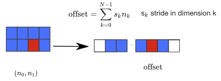
a = np.array(..)
a.flags- Various information about memory layout.a.strides- Bytes to step in each dimension when traversing.a.itemsize- Size of one array element in bytes.a.data- Python buffer object pointing to start of arrays data.a.__array_interface__- Python internal interface.
This should be familiar, so feel free to check out the NumPy documentation for more utilisation of functions.
Vetorisation
We should all be familiar with for loops in Python, and its reputation. Ideally we should be using vectorisation, which begs the question… why?
- for loops in Python are very slow
- vectorisation is an example of a SIMD operation
- one instruction carries out many operands in parallel
- less overhead compared to for loops
Lets look at a difference example:
def loop_it(n):
    t0 = time.time()
    arr = np.arange(n)
    dif = np.zeros(n-1, int)
    for i in range(1, len(arr)):
        dif[i-1] = arr[i] - arr[i-1]
    t1 = time.time()
    print('Loop version: {} seconds'.format(t1-t0))
    return dif

def vectorise_it(n):
    t0 = time.time()
    arr = np.arange(n)
    dif = arr[1:] - arr[:-1]
    t1 = time.time()
    print('Vectorised version: {} seconds'.format(t1-t0))
    return dif

n=10000000
loop_it(n)
vectorise_it(n)
Loop version: 4.1977081298828125 seconds
Vectorised version: 0.02220916748046875 seconds
array([1, 1, 1, ..., 1, 1, 1])
Arrays, slicing and powers array
Head to the Jupyter notebook and do the NumPy exercises.
Solution
Head to the solutions notebook.
Caching
You may ask… what is the cache? The cache is a part of the computer’s memory. Caching can provide an application performance boost as it is faster to access data from the temporary location than it is to fetch the data from the source each time. A computer’s memory can consists of three elements
- Main memory (RAM or ROM):
- Secondary memory
- Cache: Acts as a buffer betwwen the CPU and main memory, used to hold parts of data and program most frequently used by the CPU.
There are a few main rules of caching:
- If a function is frequently called, its output is not changing often and it takes a long time to execute, it is a suitable candidate to implement caching.
- Caching should be faster than getting the data from the current data source
- Caching impacts memory footprint, so it is crucial to choose and cache the data structures and attributes that need to be cached.
Caching itself is an optimization strategy that you can use in your applications to keep recent or often used data in memory locations that are faster to access.
The LRU (Least Recently Used) Cache discards the least recently used items first. The algorithm keeps track of what was used. The functools module deals with high-order functions, specifically:
- functions which operate on other functions
- returning functions
- other callable objects
The lru_cache() helps reduce the execution time of the function by using the memoization technique.
Let’s have a look at caching in action for the Fibonacci sequence. The least recently used algorithm can cache the return values that are dependent on the arguments that have been passed to the function.
def fib(n):
    if n < 2:
        return n
    else:
        return fib(n-1) + fib(n-2)

t1 = timeit.Timer("fib(40)", "from __main__ import fib")

print(t1.timeit(1))
27.941036257019732
from functools import lru_cache

@lru_cache(maxsize=100)
def fib(n):
    if n < 2:
        return n
    else:
        return fib(n-1) + fib(n-2)

t1 = timeit.Timer("fib(40)", "from __main__ import fib")

print(t1.timeit(1))
7.97460088506341e-05
Climbing stairs
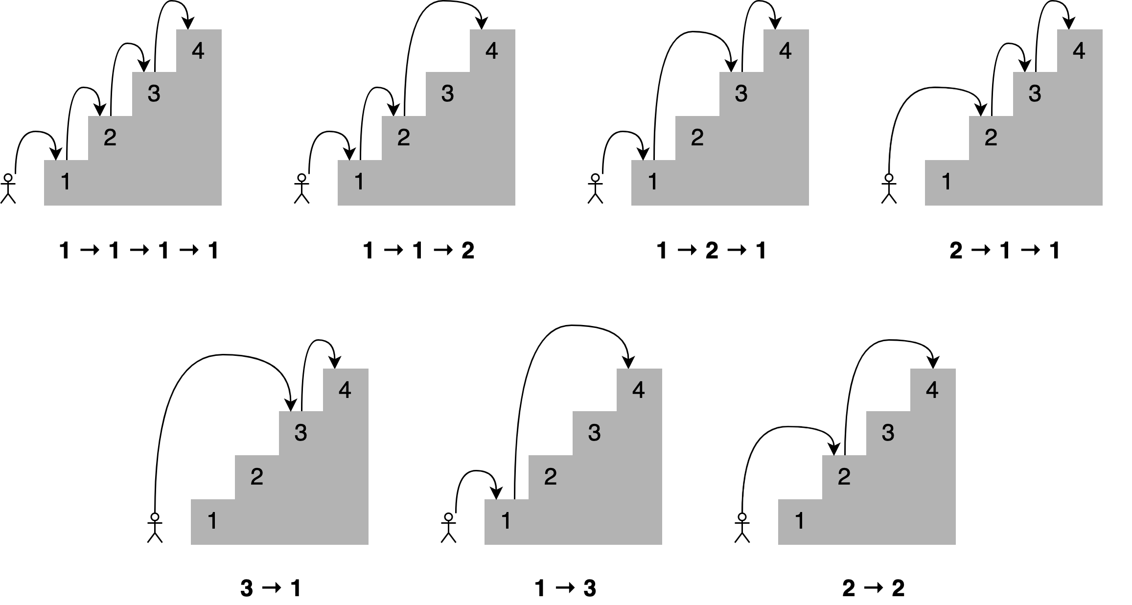
Imagine you want to determine all the different ways you can reach a specific stair in a staircase by hopping one, two, or three stairs at a time.
How many paths are there to the fourth stair? Here are all the different combinations.
A solution to this problem is to state that;
To reach your current stair, you can jump from one stair, two stairs, or three stairs below.</b>
Adding up the number of jump combinations you can use to get to each of those points should give you the total number of possible ways to reach your current position.
For 4 stairs, there are 7 combinations. For 3 there is 4, and for 2 there is 2.
The file
stairs.pyimplements recursion to solve the problem.Create a timing setup and record the time taken for 40 iterations. Then implement the lru_cache and compare the improvement.
Solution
You can find the solution in the Jupyter notebook.
Key Points
Performance code profiling is used to identify and analyse the execution and improvement of applications.
Never try and optimise your code on the first try. Get the code correct first.
Most often, about 90% of the code time is spent in 10% of the application.
The
lru_cache()helps reduce the execution time of the function by using the memoization technique, discarding least recently used items first.
Numba
Overview
Teaching: 50 min
Exercises: 25 minQuestions
What is Just-In-Time compilation
How can I implement Numba
Objectives
Compare timings for python, NumPy and Numba
Understand the different modes and toggles of Numba
![]()
What is Numba?
The name Numba is the combination of the Mamba snake and NumPy, with Mamba being in reference to the black mamba, one of the world’s fastest snakes. Numba is a just-in-time (JIT) compiler for Python functions. Numba can, from the types of the function arguments translate the function into a specialised, fast, machine code equivalent. The basic principle is that you have a Python code written, then “wrap” it in a “jit” compiler.
Under the hood, it uses an LLVM compiler infrastructure for code generation. When utilised correctly, one can get speeds similar to C/C++ and Fortran but without having to write any code in those languages, and no C/C++ compiler is required.
It sounds great, and thankfully, fairly simple. All one has to do is apply one of the Numba decorators to your Python function. A decorator is a function that takes in a function as an argument and spits out a function. As such, it is designed to work well with NumPy arrays and is therefore very useful for scientific computing. As a result, it makes it easy to parallelise your code and use multiple threads.
It works with SIMD vectorisation to get most out of your CPU. What this means is that a single instruction can be applied to multiple data elements in parallel. Numba automatically translates some loops into vector instructions and will adapt to your CPU capabilities automatically.
And to top it off, as it works with threading, you can run Numba code on GPU. This will not be covered in this lesson however, but we will cover GPUs in a later section.
When it comes to importing the correct materials, a common workflow (and one which will be replicated throughout the episode) is as follows.
import numba
from numba import jit, njit

print(numba.__version__)
It is very important to check the version of Numba that you have, as it is a rapidly evolving
library with many changes happening on a regular basis. In your own time, it is best to have an environment set up with
numba and update it regularly. We will be covering the jit and njit operators in the upcoming section.
The JIT Compiler Options/Toggles
Below we have a JIT decorator and as you can see there are plenty of different toggles and operations which we will go through.
@numba.jit(signature=None, nopython=False, nogil=False, cache=False, forceobj=False, parallel=False,
           error_model='python', fastmath=False, locals={}, boundscheck=False)
Looks like a lot, but let’s go through the different options.
-
signature: The expected types and signatures of function arguments and return values. This is known as an “Eager Compilation”. -
Modes: Numba has two modes;
nopython,forcobj. Numba will infer the argument types at call time, and generate optimized code based on this information. If there is python object, the object mode will be used by default. -
nogil=True: Releases the global interpreter lock inside the compiled function. This is one of the main reasons python is considered as slow. However this only applies innopythonmode at present. -
cache=True: Enables a file-based cache to shorten compilation times when the function was already compiled in a previous invocation. It cannot be used in conjunction withparallel=True. -
parallel=True: Enables the automatic parallelization of a number of common Numpy constructs. -
error_model: This controls the divide-by-zero behavior. Setting it topythoncauses divide-by-zero to raise an exception. Setting it tonumpycauses it to set the result to +/- infinity orNaN. -
fastmath=True: This enables the use of otherwise unsafe floating point transforms as described in the LLVM documentation. -
localsdictionary: This is used to force the types and signatures of particular local variables. It is however recommended to let Numba’s compiler infer the types of local variables by itself. -
boundscheck=True: This enables bounds checking for array indices. Out of bounds accesses will raise anIndexError. Enabling bounds checking will slow down typical functions, so it is recommended to only use this flag for debugging.
Comparing pure Python and NumPy, with and without decorators
Let us look at an example using the MonteCarlo method.
#@jit
def pi_montecarlo_python(n):
    in_circle = 0
    for i in range(int(n)):
        x, y = np.random.random(), np.random.random()
        if x ** 2 + y ** 2 <= 1.0:
            in_circle += 1

    return 4.0 * in_circle / n

#@jit
def pi_montecarlo_numpy(n):
    in_circle = 0
    x = np.random.random(int(n))
    y = np.random.random(int(n))
    in_circle = np.sum((x ** 2 + y ** 2) <= 1.0)

    return 4.0 * in_circle / n

n = 1000

print('python')
%time pi_montecarlo_python(n)
print("")
print('numpy')
%time pi_montecarlo_numpy(n)
python
CPU times: user 596 µs, sys: 1.69 ms, total: 2.29 ms
Wall time: 1.97 ms

numpy
CPU times: user 548 µs, sys: 0 ns, total: 548 µs
Wall time: 1.39 ms
Adding the jit decorators
Now, uncomment the lines with
#@jit, and run it again. What execution times do you get, and do they improve with a second run? Try reloading the function for a larger sample size. What difference do you get between normal code and code which has@jitdecorators.Output
python jit
CPU times: user 121 ms, sys: 9.4 ms, total: 131 ms
Wall time: 126 ms

numpy jit
CPU times: user 177 ms, sys: 1.85 ms, total: 179 ms
Wall time: 177 ms

SECOND RUN

python jit
CPU times: user 13 µs, sys: 5 ns, total: 18 µs
Wall time: 23.1 µs

numpy jit
CPU times: user 0 µs, sys: 21 µs, total: 21 µs
Wall time: 24.6 µs
You should have noticed that the wall time for the first run with the
@jitdecorators was significantly slower than the original code. Then, when we run it again, it is much quicker So what’s going on?
The decorator is taking the python function and translating it into fast machine code, it will naturally take more time to do so. This compilation time, is the time for numba to look through your code and translate it. If you are using a slow function and only using it once, then Numba will only slow it down. Therefore, Numba is best used for functions that you will be repeatedly using throughout your program.
Once the compilation has taken place Numba caches the machine code version of the function for the particular types of
arguments presented, for example if we changed n to 1000.0 as a floating point number, we will get a longer execution
time again, as the machine code has had to be rewritten.
To benchmark Numba-compiled functions, it is important to time them without including the compilation step.
The compilation will only happen once for each set of input types, but the function will be called many times. By
adding @jit decorator we see major speed ups for Python and a bit for NumPy. Numba is very useful in speeding up
python loops that cannot be converted to NumPy or it’s too complicated. NumPy can sometimes reduce readability. We can
therefore get significant speed ups with minimum effort.
Demonstrating modes
nopython=True
Below we have a small function that determines whether a function is a prime number, then generate an array of random
numbers. We are going to use a decorator for this example, which itself is a function that takes another function as
its argument, and returns another function, defined by is_prime_jit. This is as an alternative to using @jit.
def is_prime(n):
    if n <= 1:
        raise ArithmeticError('%s <= 1' %n)
    if n == 2 or n == 3:
        return True
    elif n % 2 == 0:
        return False
    else:
        n_sqrt = math.ceil(math.sqrt(n))
        for i in range(3, n_sqrt):
            if n % i == 0:
                return False

    return True

numbers = np.random.randint(2, 100000, size=10)

is_prime_jit = jit(is_prime)
Now we will time and run the function with pure python, jitted including compilation time and then purely with jit. Take note of the timing setup, as you will use this regularly through the episode.
print("Pure Python")
%time p1 = [is_prime(x) for x in numbers]
print("")
print("Jitted including compilation")
%time p2 = [is_prime_jit(x) for x in numbers]
print("")
print("Jitted")
%time p2 = [is_prime_jit(x) for x in numbers]
Warning explanation
Upon running this, you will get an output with a large warning, amongst it will say,
Pure Python
CPU times: user 798 µs, sys: 0 ns, total: 798 µs
Wall time: 723 µs

Jitted including compilation
...
... Compilation is falling back to object with WITH looplifting enabled because Internal error in pre-inference
rewriting pass encountered during compilation of function "is_prime" due to ...
...

CPU times: user 482 ms, sys: 16.9 ms, total: 499 ms
Wall time: 496 ms

Jitted
CPU times: user 43 µs, sys: 0 ns, total: 43 µs
Wall time: 46 µs
This still runs as we would expect, and if we run it again, the warning disappears.
If we change the above code and add one of our toggles so that the jitted line becomes;
is_prime_jit = jit(nopython=True)(is_prime)
We will get a full error, because it CANNOT run in nopython mode. However, by setting this mode to True, you
can highlight where in the code you need to speed it up. So how can we fix it?
If we refer back to the code, and the error, it arises in the notation in Line 3 for the ArithmeticError, or more
specifically '%s <= 1'. This is a python notation, and to translate it into pure machine code, it needs the python
interpreter. We can change it to 'n <= 1', and when rerun we get no warnings or error.
Although what we have just done is possible without nopython, it is a bit slower, and worth bearing in mind.
@jit(nopython=True) is equivalent to @njit. The behaviour of the nopython compilation mode is to essentially
compile the decorated function so that it will run entirely without the involvement of the Python interpreter. If it
can’t do that an exception is raised. These exceptions usually indicate places in the function that need to be modified
in order to achieve better-than-Python performance. Therefore, we strongly recommend always using nopython=True. This
supports a subset of python but runs at C/C++/Fortran speeds.
Object mode (forceobj=True) extracts loops and compiles them in nopython mode which useful for functions that are
bookended by uncompilable code but have a compilable core loop, this is also done automatically. It supports nearly all
of python but cannot speed up by a large factor.
Mandelbrot example
Let’s now create an example of the Mandelbrot set, or strictly speaking, a Julia set in reality. We won’t go into
full details on what is going on in the code, but there is a while loop in the kernel function that is causing this
to be slow as well as a couple of for loops in the compute_mandel_py function.
import numpy as np
import math
import time
import numba
from numba import jit, njit
import matplotlib.pyplot as plt

mandel_timings = []

def plot_mandel(mandel):
    fig=plt.figure(figsize=(10,10))
    ax = fig.add_subplot(111)
    ax.set_aspect('equal')
    ax.axis('off')
    ax.imshow(mandel, cmap='gnuplot')
    plt.savefig('mandel.png')

def kernel(zr, zi, cr, ci, radius, num_iters):
    count = 0
    while ((zr*zr + zi*zi) < (radius*radius)) and count < num_iters:
        zr, zi = zr * zr - zi * zi + cr, 2 * zr * zi + ci
        count += 1
    return count

def compute_mandel_py(cr, ci, N, bound, radius=1000.):
    t0 = time.time()
    mandel = np.empty((N, N), dtype=int)
    grid_x = np.linspace(-bound, bound, N)

    for i, x in enumerate(grid_x):
        for j, y in enumerate(grid_x):
            mandel[i,j] = kernel(x, y, cr, ci, radius, N)
    return mandel, time.time() - t0

def python_run():
    kwargs = dict(cr=0.3852, ci=-0.2026,
              N=400,
              bound=1.2)
    print("Using pure Python")
    mandel_func = compute_mandel_py
    mandel_set = mandel_set, runtime = mandel_func(**kwargs)

    print("Mandelbrot set generated in {} seconds".format(runtime))
    plot_mandel(mandel_set)
    mandel_timings.append(runtime)

python_run()

print(mandel_timings)
For larger values of N in python_run, we recommend submitting this to the compute nodes. For more information on
submitting jobs on an HPC, you can consult our intro-to-hpc course.
For the moment however we can provide you with the job script in an exercise.
Submit a job to the queue
Below is a job script that we have prepared for you. All you need to do is run it! This script will run the code above, which can be written to a file called
mandel.py. Your instructor will inform you of the variables to use in the values$ACCOUNT,$PARTITION, and$RESERVATION.#!/bin/bash #SBATCH --nodes=1 #SBATCH --time=00:10:00 #SBATCH -A $ACCOUNT #SBATCH --job-name=mandel #SBATCH -p $PARTITION #SBATCH --reservation=$RESERVATION module purge module load conda module list source activate numba cd $SLURM_SUBMIT_DIR python mandel.py exit 0To submit the job, you will need the following command. It will return a job ID.
$ sbatch mandel_job.shOnce the job has run successfully, run it again but this time, use
njiton thekernelfunction.Output
Check the directory where you submitted the command and you will have a file called
slurm-123456.out, where the123456will be replaced with your job ID as returned in the previous example. View the contents of the file and it will give you an output returning the time taken for the mandelbrot set. ForN = 400it will be roughly 10-15 seconds. A.pngfile will also be generated.To view the
njitsolution, head to the file here.
Now, let’s see if we can speed it up more by looking at the compute function.
compute_mandel_njit_jit = njit()(compute_mandel_njit)

def njit_njit_run():
    kwargs = dict(cr=0.3852, ci=-0.2026,
              N=400,
              bound=1.2)
    print("Using njit kernel and njit compute")
    mandel_func = compute_mandel_njit_jit
    mandel_set = mandel_set, runtime = mandel_func(**kwargs)

    print("Mandelbrot set generated in {} seconds".format(runtime))

njit_njit_run()
njitthe compute functionAdd the modifications to your code and submit the job. What kind of speed up do you get?
Solution
Not even a speed-up, an error, because there are items in that function that Numba does not like! More specifically if we look at the error;
...
Unknown attribute 'time' of type Module ...
...
This is a python object, so we need to remove the
time.timefunction.
Now let’s modify the code to ensure it is timed outside of the main functions. Running it again will produce another error about data types, so these will also need to be fixed.
Fix the errors!
Change all the instances of
dtype=inttodtype=np.int_incompute_mandelfunctions throughout.Solution
import matplotlib.pyplot as plt

mandel_timings = []

def plot_mandel(mandel):
    fig=plt.figure(figsize=(10,10))
    ax = fig.add_subplot(111)
    ax.set_aspect('equal')
    ax.axis('off')
    ax.imshow(mandel, cmap='gnuplot')

def kernel(zr, zi, cr, ci, radius, num_iters):
    count = 0
    while ((zr*zr + zi*zi) < (radius*radius)) and count < num_iters:
        zr, zi = zr * zr - zi * zi + cr, 2 * zr * zi + ci
        count += 1
    return count

kernel_njit = njit(kernel)

def compute_mandel_njit(cr, ci, N, bound, radius=1000.):
    mandel = np.empty((N, N), dtype=np.int_)
    grid_x = np.linspace(-bound, bound, N)

    for i, x in enumerate(grid_x):
        for j, y in enumerate(grid_x):
            mandel[i,j] = kernel_njit(x, y, cr, ci, radius, N)
    return mandel

compute_mandel_njit_jit = njit()(compute_mandel_njit)

def njit_njit_run():
    kwargs = dict(cr=0.3852, ci=-0.2026,
              N=200,
              bound=1.2)
    print("Using njit kernel and njit compute")
    mandel_func = compute_mandel_njit_jit
    mandel_set = mandel_func(**kwargs)

    plot_mandel(mandel_set)

njit_njit_run()
We recommend trying this out in the Jupyter notebook as well for your own reference
t0 = time.time()
njit_njit_run()
runtime = time.time() - t0
mandel_timings.append(runtime)
print(mandel_timings)
cache=True
The point of using cache=True is to avoid repeating the compile time of large and complex functions at each run of a
script. In the example below the function is simple and the time saving is limited but for a script with a number of
more complex functions, using cache can significantly reduce the run-time. We have removed the python object that
caused the error. We will switch back to the is_prime function here.
def is_prime(n):
    if n <= 1:
        raise ArithmeticError('n <= 1')
    if n == 2 or n == 3:
        return True
    elif n % 2 == 0:
        return False
    else:
        n_sqrt = math.ceil(math.sqrt(n))
        for i in range(3, n_sqrt):
            if n % i == 0:
                return False

    return True

is_prime_njit = njit()(is_prime)
is_prime_njit_cached = njit(cache=True)(is_prime)

numbers = np.random.randint(2, 100000, size=1000)
Compare the timings for
cacheRun the function 4 times so that you get results for:
- Not cached including compilation
- Not cached
- Cached including compilation
- Cached
Output
You may get a result similar to below.
Not cached including compilation
CPU times: user 117 ms, sys: 11.7 ms, total: 128 ms
Wall time: 134 ms

Not cached
CPU times: user 0 ns, sys: 381 µs, total: 381 µs
Wall time: 386 µs

Cached including compilation
CPU times: user 2.84 ms, sys: 1.95 ms, total: 4.79 ms
Wall time: 11.8 ms

Cached
CPU times: user 378 µs, sys: 0 ns, total: 378 µs
Wall time: 382 µs
It may not be as fast as when its been compiled in the same environment you are running your program in, but can still be a considerable speed up for bigger scripts. Usually to show the cache working, you need to restart the whole kernel and subsequently reload the modules, functions and variables.
Eager Compilation using function signatures
This speeds up compilation time faster than cache, hence the term “eager”. It can be helpful if you know the types of input and output values of your function before you compile it. Although python can be fairly lenient if you are not concerned about types, at the machine level it makes a big difference. We will look more into the importance of typing in upcoming episodes, but for now, let’s look again at our prime example. We do not need to edit the code itself, merely the njit.
To enable eager compilation, we need to specify the input and output types. For is_prime, the output is a boolean,
and the input is an integer, we have to specify that as well. It needs to be declared in the form output(input).
Types should be ordered from smaller to higher precision, i.e. int32, int64. We have to cover for both methods of
precision.
is_prime_eager = njit(['boolean(int32)','boolean(int64)' ])(is_prime)
Compare the timings for eager compilation
Run the function 4 times so that you get results for:
- Just njit including compilation
- Just njit
- Eager including compilation
- Eager
Output
You may expect an output similar to the following.
Just njit including compilation
CPU times: user 97.2 ms, sys: 2.19 ms, total: 99.4 ms
Wall time: 100 ms

Just njit
CPU times: user 3.6 ms, sys: 0 ns, total: 3.6 ms
Wall time: 3.48 ms

Eager including compilation
CPU times: user 3.61 ms, sys: 0 ns, total: 3.61 ms
Wall time: 3.57 ms

Eager
CPU times: user 3.42 ms, sys: 367 µs, total: 3.79 ms
Wall time: 3.64 ms
Bear in mind these are small examples, but you can clearly see how much time that has shaved off this small example .
fastmath=True
The final one we will look at for is_prime is fastmath=True. This enables the use of otherwise unsafe floating
point transforms. This means that it is possible to relax some numerical rigour with view of gaining additional
performance. As an example, it assumes that the arguments and result are not NaN or infinity values. Feel free to
investigate the llvm docs. The key thing with this toggle is that
you have to be confident with the inputs of your code and that there is no chance of returning NaN or infinity.
is_prime_njit_fmath = njit(fastmath=True)(is_prime)
Running this, you may expect an timings output similar to below.
CPU times: user 3.75 ms, sys: 0 ns, total: 3.75 ms
Wall time: 3.75 ms

Fastmath including compilation
CPU times: user 96 ms, sys: 477 µs, total: 96.5 ms
Wall time: 93.9 ms

Fastmath compilation
CPU times: user 3.5 ms, sys: 0 ns, total: 3.5 ms
Wall time: 3.41 ms
Toggling with toggles with Montecarlo
Head to the Numba Exercise Jupyter notebook and work on Exercise 2. You should try out
@njit, eager compilation,cacheandfastmathon the MonteCarlo function and compare the timings you get. Feel free to submit larger jobs to the queue.Solution
The solution can be found in the notebook here.
parallel=True
We can also use Numba to parallelise our code by using parallel=True to use multi-core CPUs via threading. We can use
numba.prange alongside parallel=True if you have for loops present in your code. As a default, the option is set to
False, and doing so means that numba.prange has the same utility as range. We can set the default number of
threads with the following syntax.
max_threads = numba.config.NUMBA_NUM_THREADS
def pi_montecarlo_python(n):
    in_circle = 0
    for i in range(n):
        x, y = np.random.random(), np.random.random()
        if x ** 2 + y ** 2 <= 1.0:
            in_circle += 1

    return 4.0 * in_circle / n

def pi_montecarlo_numpy(n):
    in_circle = 0
    x = np.random.random(n)
    y = np.random.random(n)
    in_circle = np.sum((x ** 2 + y ** 2) <= 1.0)

    return 4.0 * in_circle / n

n = 1000000

pi_montecarlo_python_njit = njit()(pi_montecarlo_python)

pi_montecarlo_numpy_njit = njit()(pi_montecarlo_numpy)

pi_montecarlo_python_parallel = njit(parallel=True)(pi_montecarlo_python)

pi_montecarlo_numpy_parallel = njit(parallel=True)(pi_montecarlo_numpy)
If the pure python version seems faster than numpy, there is no need for concern, as sometimes python + numba can turn out to be faster than numpy + numba.
Explaining warnings
If you run the above code, you may see that you get a warning saying:
...
The keyword argument 'parallel=True' was specified but no transformation for parallel executing code was possible.
...
Running it again will remove the warning, but we will not get any speed-up. We will need to change the above code in Line 3 from
for i in range(n):tofor i in numba.prange(n):.
njit_python including compilation
CPU times: user 105 ms, sys: 4.66 ms, total: 110 ms
Wall time: 105 ms

njit_python
CPU times: user 10.1 ms, sys: 0 ns, total: 10.1 ms
Wall time: 9.93 ms

njit_numpy including compilation
CPU times: user 174 ms, sys: 7.61 ms, total: 181 ms
Wall time: 179 ms

njit_numpy
CPU times: user 11.1 ms, sys: 4.3 ms, total: 15.4 ms
Wall time: 15.2 ms

njit_python_parallel including compilation
CPU times: user 536 ms, sys: 29.1 ms, total: 565 ms
Wall time: 480 ms

njit_python_parallel
CPU times: user 60.3 ms, sys: 8.65 ms, total: 68.9 ms
Wall time: 3.2 ms

njit_numpy_parallel including compilation
CPU times: user 3.89 s, sys: 726 ms, total: 4.62 s
Wall time: 789 s

njit_numpy_parallel
CPU times: user 53.1 ms, sys: 9.96 ms, total: 63 ms
Wall time: 2.77 ms
Set the number of threads
Increase the value of N and adjust the number of threads using
numba.set_num_threads(nthreads). What sort of timings do you get. Are they what you would expect? Why?
Diagnostics
Using the command below:
pi_montecarlo_numpy_parallel.parallel_diagnostics(level=N)You can get an understanding of what is going on under the hood. You can replace the value N for numbers between 1 and 4.
Creating ufuncs using numba.vectorize
A universal function (or ufunc for short) is a function that operates on ndarrays in an element-by-element fashion.
So far we have been looking at just-in-time wrappers, these are “vectorized” wrappers for a function. For example
np.add() is a ufunc.
There are two main types of ufuncs:
- Those which operate on scalars, ufuncs (see
@vectorizebelow). - Those which operate on higher dimensional arrays and scalars, these are “generalized universal functions” or gufuncs,
such as
@guvectorize.
The @vectorize decorator allows Python functions taking scalar input arguments to be used as NumPy ufuncs. Creating
a traditional NumPy ufunc involves writing some C code. Thankfully, Numba makes this easy. This decorator means Numba
can compile a pure Python function into a ufunc that operates over NumPy arrays as fast as traditional ufuncs written
in C.
The vectorize() decorator has two modes of operation:
- Eager, or decoration-time, compilation: If you pass one or more type signatures to the decorator, you will be building a Numpy universal function (ufunc). It is passed in the formw
output_type1(input_type1)
output_type2(input_type12)
# etc
- Lazy, or call-time, compilation: When not given any signatures, the decorator will give you a Numba dynamic universal function (DUFunc) that dynamically compiles a new kernel when called with a previously unsupported input type.
If you pass several signatures, beware that you have to pass the more specific signatures before least specific ones
(e.g., single-precision floats before double-precision floats), otherwise type-based dispatching will not work as
expected. eg (int32,int64,float32,float64)
Here is a very simple example one with vectorization and the other with parallelisation as well.
numba.set_num_threads(max_threads)

def numpy_sin(a, b):
    return np.sin(a) + np.sin(b) + np.cos(a) - np.cos(b) + (np.sin(a))**2


numpy_sin_vec = numba.vectorize(['int64(int64, int64)','float64(float64, float64)'])(numpy_sin)

numpy_sin_vec_par = numba.vectorize(['int64(int64, int64)','float64(float64, float64)'],target='parallel')(numpy_sin)

x = np.random.randint(0, 100, size=90000)
y = np.random.randint(0, 100, size=90000)

print("Just numpy")
%time _ = numpy_sin(x, y)
print("")
print("Vectorised")
%time _ = numpy_sin_vec(x, y)
print("")
print("Vectorised & parallelised")
%time _ = numpy_sin_vec_par(x, y)
Just numpy
CPU times: user 17.3 ms, sys: 4.08 ms, total: 21.4 ms
Wall time: 20.1 ms

Vectorised
CPU times: user 14.9 ms, sys: 0 ns, total: 14.9 ms
Wall time: 14.5 ms

Vectorised & parallelised
CPU times: user 86.5 ms, sys: 18.7 ms, total: 105 ms
Wall time: 8.72 ms
Vectorisation
Head to the Jupyter notebook and Exercise 3. Work on the
is_primefunction by utilisingnjit,vectorizeand then vectorize it with the target set toparallel. Time the results and compare the output.Solution
The solution can be found in the notebook here.
Key Points
Numba only compiles individual functions rather than entire scripts.
The recommended modes are
nopython=TrueandnjitNumba is constantly changing, so keep checking for new versions.
Cython
Overview
Teaching: 45 min
Exercises: 60 minQuestions
What is Cython?
What’s happening under the hood?
How can I implement a Cython workflow?
How can I create C-type declarations?
Objectives
To understand the main concepts of C relative to Cython
Learn how to implement a Cython workflow in a Jupyter notebook and in a terminal environment]9oii
Implement type declarations across variables and functions, as well as compiler directives
Undertake a Julia-set example
![]()
What is Cython?
Cython is a programming language that makes writing C extensions for the Python language as easy as Python itself. The source code gets translated into optimised C/C++ code and compiled as Python extension modules. The code is executed in the CPython runtime environment, but at the speed of compiled C with the ability to call directly into C libraries, whilst keeping the original interface of the Python source code.
This enables Cython’s two major use cases:
- Extending the CPython interpreter with fast binary modules
- Interfacing Python code with external C libraries
An important thing to remember is that Cython IS Python, only with C data types, so lets take a little but of time to get into some datatypes.
Typing
Cython supports static type declarations, thereby turning readable Python code into plain C performance. There are two main recognised ways of “typing”.
Static Typing
Type checking is performed during compile-time. For example, the expression x = 4 + 'e' would not compile. This
method of typing can detect type errors in rarely used code paths
Dynamic Typing
In contrast, type checking is performed during run-time. Here, the expression x = 4 + 'e' would result in a runtime
type error. This allows for fast program execution and tight integration with external C libraries.
Datatype declarations
Python is a programming language with an exception to the normal rule of datatype declaration. Across most programming languages you will see variables associated with a specific type, such as integers (
int), floats (float,double), and strings (str).We see datatypes used in pure Python when declaring things as a
listordict. For most Cython operations we will be doing the same for all variable types.
Implementing Cython
This can be implemetned either by Cython scripts or by using cell magics (%%) in Jupyter notebooks. Although the
notebooks are available, we also recommend trying these methods outside the notebook, as it is the more commonly used
implementation. You can use Jupyter notebooks to create external files as an alternative.
Using Jupyter Notebook cell magics with Cython
As discussed in episode 2, we can use cell magics to implement Cython in Jupyter notebooks. The first cell magic that we need is to load Cython itself. This can be done with a separate cell block that only needs to be run once in the notebook.
%load_ext cythonFrom there, any cell that we wish to “cythonise” needs to have the following on the first line of any cell.
%%cython

# Some stuff
Let’s look at how to cythonise a simple function which calculates the Fibonacci sequence for a given set of numbers,
n. Below we have the python code for a file which we have named fibonacci.py.
def fib(n):
    # Prints the Fibonacci series up to n.
    a, b = 0, 1
    while b < n:
        print(b)
        a, b = b, a + b
Although we are only dealing with one file here, it is common practice to have a “main” file from which all other files
and functions are called. This may seem unnecessary for this simple setup, but is good practice, particularly when you
have a setup that has dozens, hundreds of functions. We will create a simple fibonacci_main.py file which imports the
fib function, then runs it with a fixed value for n.
from fibonacci import fib

fib(10)
From here we can run the file in the terminal, or if you are using Jupyter notebook, you can use the cells themselves,
or use the ! operator to implement bash in the codeblock.
$ python fibonacci_main.py
That’s our Python setup, now let’s go about cythonising it. We will use the same function as before, but now we will
save it as a .pyx file. It can be helpful when dealing with Cython to rename your functions accordingly, as we can
see below.
def fib_cyt(n):
    # Prints the Fibonacci series up to n.
    a, b = 0, 1
    while b < n:
        print(b)
        a, b = b, a + b
Before we change our fibonacci_main.py to implement the function using Cython, we need to ado a few more things.
This .pyx file is compiled by Cython into a .c file, which itself is then compiled by a C compiler to a .so or
.dylib file. We will learn a bit more about these different file types in the
next episode.
There are a few different ways to build your extension module. We are going to look at a method which creates a file
which we will call setup_fib.py, which “cythonises” the file. It can be viewed as the Makefile of python. In it, we
need to import some modules and call a function which enables us to setup the file.
from distutils.core import setup, Extension
from Cython.Build import cythonize

setup(ext_modules = cythonize("fibonacci_cyt.pyx"))
Let us have a look at the contents of our current working directory, and see how it changes as we run this setup file.
$ ls
04-Cython.ipynb   exercise          fibonacci_cyt.pyx setup_fib.py
__pycache__       fibonacci.py      fibonacci_main.py
At this stage all we have are our original Python files, our .pyx file and setup_fib.py. Now lets run our
setup_fib.py and see how that changes.
In the terminal (or by using ! in notebook), we will now build the extension to use in the current working directory.
You should get a printed message to the screen, now let’s check the output of ls to see how our directory has changed.
04-Cython.ipynb                    fibonacci_cyt.c
__pycache__                        fibonacci_cyt.cpython-38-darwin.so
build                              fibonacci_cyt.pyx
exercise                           fibonacci_main.py
fibonacci.py                       setup_fib.py
So, a few more things have been added now.
- The
.cfile, which is then compiled using a C compiler - The
build/directory, which contains the.ofile generated by the compiler - The
.soor.dylibfile. This is the compiled library
Next we add the main file which we will use to run our program. We can call it fibonacci_cyt_main.py.
from fibonacci_cyt import fib_cyt

fib_cyt(10)
Upon running it, you can see that it works the same as our regular version. We will get into ways on how to speed up the code itself shortly.
Compiling an addition module
Define a simple addition module below, which containing the following function, and write it to a file called
cython_addition.pyx.Modify it to return x + y.def addition(x, y): # TODOUtilise the function by importing it into a new file,
addition_main.py. Edit thesetup.pyaccordingly to import the correct file. Use the demo above as a reference.Solution
cython_addition.pyxdef addition(x, y): print(x + y)
addition_main.pyfrom cython_addition import addition addition(2,3)
setup.pyfrom distutils.core import setup, Extension from Cython.Build import cythonize setup(ext_modules = cythonize("cython_addition.pyx"))$ python setup.py build_ext --inplace $ python addition_main.py
Accelerating Cython
Compiling with Cython is fine, but it doesn’t speed up our code to actually make a significant difference. We need to implement the C-features that Cython was designed for. Let’s take the code block below as an example of some code to speed up.
import time
from random import random

def pi_montecarlo(n=1000):
    '''Calculate PI using Monte Carlo method'''
    in_circle = 0
    for i in range(n):
        x, y = random(), random()
        if x ** 2 + y ** 2 <= 1.0:
            in_circle += 1

    return 4.0 * in_circle / n

N = 100000000

t0 = time.time()
pi_approx = pi_montecarlo(N)
t_python = time.time() - t0
print("Pi Estimate:", pi_approx)
print("Time Taken", t_python)
Running this as a .py file for 100,000,000 points will result in a time of ~27.98 seconds. Compiling with Cython
will speed it up to ~17.20 seconds.
It may be a speed-up but not as significant as we would want. There are a number of different methods we can use.
Static type declarations
These allow Cython to step out of the dynamic nature of the Python code and generate simpler and faster C code, and sometimes it can make code faster by orders of magnitude.
This is often the simplest and quickest way to achieve significant speedup, but trade-off is that the code can become more verbose and less readable.
Types are declared with cdef keyword. Now let’s implement this into our montecarlo file.
def pi_montecarlo(int n=1000):
    cdef int in_circle = 0, i
    cdef double x, y
    for i in range(n):
        x, y = random(), random()
        if x ** 2 + y ** 2 <= 1.0:
            in_circle += 1

    return 4.0 * in_circle / n
Running this using the timing setup from the previous code block, by only declaring our variables as an int and
double has decreased our execution time to ~4.03 seconds.
We can go further though!
Typing function calls
As with ‘typing’ variables, you can also ‘type’ functions. Function calls in Python can be expensive, and can be even more expensive in Cython as one might need to convert to and from Python objects to do the call.
There are two ways in which to declare C-style functions in Cython;
- Declaring a C-type function with
cdef. This is the same as declaring a variable - Creating a Python wrapper with
cpdef
Using
cdefandcpdefin notebooks with magicsA side-effect of
cdefis that the function is no longer available from Python-space, so Python won’t know how to call it.If we declare a simple function like below in a Jupyter notebook cell;
cdef double cube_cdef(double x):
    return x ** 3
And from there we use
%time cube_cdef(3), we will get the following error.--------------------------------------------------------------------------- NameError Traceback (most recent call last) <timed eval> in <module> NameError: name 'cube_cdef' is not definedIf we want to be able to use the magics command, we will need to use
cpdef.
Now let’s implement our function call.
cdef double pi_montecarlo(int n=1000):
    '''Calculate PI using Monte Carlo method'''
    cdef int in_circle = 0, i
    cdef double x, y
    for i in range(n):
        x, y = random(), random()
        if x ** 2 + y ** 2 <= 1.0:
            in_circle += 1

    return 4.0 * in_circle / n
Our timing has reduced again to ~3.60 seconds. Not a massive decrease, but still significant.
Static type declarations and function call overheads can significantly reduce runtime, however there are additional things you can do to significantly speed up runtime.
NumPy arrays with Cython
Let’s take a new example with a numpy array that calculates a 2D array.
import numpy as np
def powers_array(N, M):
    data = np.arange(M).reshape(N,N)

    for i in range(N):
        for j in range(N):
            data[i,j] = i**j
    return(data[2])

%time powers_array(15, 225)
CPU times: user 159 µs, sys: 112 µs, total: 271 µs
Wall time: 294 µs
array([    1,     2,     4,     8,    16,    32,    64,   128,   256,
         512,  1024,  2048,  4096,  8192, 16384])
A small function that takes a short amount of time, but there is a NumPy array we can cythonise. We need to import
NumPy with cimport then declare it as a C variable.
import numpy as np # Normal NumPy import
cimport numpy as cnp # Import for NumPY C-API

def powers_array_cy(int N, int M): # declarations can be made only in function scope
    cdef cnp.ndarray[cnp.int_t, ndim=2] data
    data = np.arange(M).reshape((N, N))


    for i in range(N):
        for j in range(N):
            data[i,j] = i**j
    return(data[2])

%time powers_array_cy(15,225)
CPU times: user 151 µs, sys: 123 µs, total: 274 µs
Wall time: 268 µs
array([    1,     2,     4,     8,    16,    32,    64,   128,   256,
         512,  1024,  2048,  4096,  8192, 16384])
Note that for a small array like this, the speed up is not significant, you may even have got a slow down, why? Have a think as we go through the final main step on how to speed up code.
For larger problems with larger arrays, speeding up code using cnp arrays are recommended!
Compiler directives
These affect the code in a way to get the compiler to ignore things that it would usually look out for. There are plenty of examples as discussed in the Cython documentation, however the main ones we will use here are;
boundscheck- If set toFalse, Cython is free to assume that indexing operations in the code will not cause any IndexErrors to be raisedwraparound- If set toFalse, Cython is allowed to neither check for nor correctly handle negative indices. This can cause data corruption or segmentation faults if mishandled, so use with caution!
You should implement these at a point where you know that the code is working efficiently and that any issues what could be raised by the compiler are sorted. There are a few ways to implement them;
- With a header comment at the top of a
.pyxfile, which must appear before any code
# cython: boundscheck=False
- Passing a directive on the command line using the -X switch
$ cython -X boundscheck=True ...
- Or locally for specific functions, for which you first need the cython module imported
  cimport cython
  @cython boundscheck(False)
Let’s see how this applies in our powers example.
import numpy as np # Normal NumPy import
cimport numpy as cnp # Import for NumPY C-API

cimport cython

@cython.boundscheck(False) # turns off
@cython.wraparound(False)

def powers_array_cy(int N, int power): # number of
    cdef cnp.ndarray[cnp.int_t, ndim=2] arr
    cdef int M
    M = N*N
    arr = np.arange(M).reshape((N, N))

    for i in range(N):
        for j in range(N):
            arr[i,j] = i**j
    return(arr[power]) # returns the ascending powers

%time powers_array_cy(15,4)
CPU times: user 166 µs, sys: 80 µs, total: 246 µs
Wall time: 238 µs
array([        1,         4,        16,        64,       256,      1024,
            4096,     16384,     65536,    262144,   1048576,   4194304,
        16777216,  67108864, 268435456])
Typing and Profiling
For anyone new to Cython and the concept of declaring types, there is a tendency to ‘type’ everything in sight. This reduces readability and flexibility and in certain situations, even slow things down in some circumstances, such as what we saw in the previous code block. We have unnecessary typing
It is also possible to kill performance by forgetting to ‘type’ a critical loop variable. Tools we can use are profiling and annotation.
Profiling is the first step of any optimisation effort and can tell you where the time is being spent. Cython’s annotation can tell you why your code is taking so long.
Using the -a switch in cell magics (%%cython -a), or cython -a cython_module.pyx from the terminal creates a HTML
report of Cython and generated C code. Alternatively, pass the annotate=True parameter to cythonize() in the
setup.py file (Note, you may have to delete the C file and compile again to produce the HTML report).
This HTML report will colour lines according to typeness. White lines translate to pure C (fast as normal C code).
Yellow lines are those that require the Python C-API. Lines with a + are translated to C code and can be viewed by
clicking on it.
By default, Cython code does not show up in profile produced by cProfile. In Jupyter notebook or indeed a source file, profiling can be enabled by including in the first line;
# cython: profile=True
Alternatively, if you want to do it on a function by function basis, you can exclude a specific function while profiling code.
# cython: profile=True
import cython
@cython.profile(False)
cdef func():
Or alternatively, you only need to profile a highlighted function
# cython: profile=False
import cython
@cython.profile(True)
cdef func():
To run the profile in Jupyter, we can use the cell magics %prun func()
Generate a profiling report
Use the methoda described above to profile the Montecarlo code. What lines of the code hint at a Python interaction? Why?
Acceleration Case Study: Julia Set
Now we will look at a more complex example, the Julia set. This is also covered in the Jupyter notebook.
import matplotlib.pyplot as plt
import time
import numpy as np
from numpy import random
%matplotlib inline

mandel_timings = []


def plot_mandel(mandel):
    fig=plt.figure(figsize=(10,10))
    ax = fig.add_subplot(111)
    ax.set_aspect('equal')
    ax.axis('off')
    ax.imshow(mandel, cmap='gnuplot')
    plt.savefig('mandel.png')

def kernel(zr, zi, cr, ci, radius, num_iters):
    count = 0
    while ((zr*zr + zi*zi) < (radius*radius)) and count < num_iters:
        zr, zi = zr * zr - zi * zi + cr, 2 * zr * zi + ci
        count += 1
    return count

def compute_mandel_py(cr, ci, N, bound, radius=1000.):
    t0 = time.time()
    mandel = np.empty((N, N), dtype=int)
    grid_x = np.linspace(-bound, bound, N)

    for i, x in enumerate(grid_x):
        for j, y in enumerate(grid_x):
            mandel[i,j] = kernel(x, y, cr, ci, radius, N)
    return mandel, time.time() - t0

def python_run():
    kwargs = dict(cr=0.3852, ci=-0.2026,
              N=500,
              bound=1.2)
    print("Using pure Python")
    mandel_func = compute_mandel_py
    mandel_set, runtime = mandel_func(**kwargs)
    print("Mandelbrot set generated in {} seconds\n".format(runtime))
    plot_mandel(mandel_set)
    mandel_timings.append(runtime)

%time python_run()
Using pure Python
Mandelbrot set generated in 22.584877729415894 seconds

CPU times: user 22.5 s, sys: 144 ms, total: 22.7 s
Wall time: 22.7 s

Optimise the Julia set
As mentioned, this pure python code is in need of optimisation. Conduct a step by step process to speed up the code. The steps that you take, as well as the estimated execution times for
N=500should be as follows.
- Compilation with Cython - ~ 19 seconds
- Static type declarations - ~ 0.15 seconds
- Declaration as C function - ~ 0.13 seconds
- Fast Indexing and compiler directives - ~ 0.085 seconds
- use
cimport- look at the loops, is there a faster way of doing it?
As you can see you might expect a speed up of roughly 250-300 times the original python code. The Jupyter notebook outlines the process well if you need it, but try it out yourself. The solution is the final step.
Solution
Feel free to continue experimenting, as you may still find a quicker method!
import numpy as np
import time
cimport numpy as cnp

from cython cimport boundscheck, wraparound

@wraparound(False)
@boundscheck(False)

cdef int kernel(double zr, double zi, double cr, double ci,
           double radius, int num_iters):
    cdef int count = 0
    while ((zr*zr + zi*zi) < (radius*radius)) and count < num_iters:
        zr, zi = zr * zr - zi * zi + cr, 2 * zr * zi + ci
        count += 1
    return count

def compute_mandel_cyt(cr, ci, N, bound, radius=1000.):
    t0 = time.time()

    cdef cnp.ndarray[cnp.int_t, ndim=2] mandel
    mandel = np.empty((N, N), dtype=int)

    cdef cnp.ndarray[cnp.double_t, ndim=1] grid_x
    grid_x = np.linspace(-bound, bound, N)

    cdef:
        int i, j
        double x, y

    for i in range(N):
        for j in range(N):
            x = grid_x[i]
            y = grid_x[j]

            mandel[i,j] = kernel(x, y, cr, ci, radius, N)
    return mandel, time.time() - t0
def speed_run():
    kwargs = dict(cr=0.3852, ci=-0.2026,
              N=2000,
              bound=0.12)
    mandel_func = compute_mandel_cyt
    mandel_set, runtime = mandel_func(**kwargs)
    print("Mandelbrot set generated: \n")
    print("Using advanced techniques: {}\n".format(runtime))
    plot_mandel(mandel_set)
    print("Assuming the same speed up factor, our original code would take", (speed_up_factor*runtime)/60, "minutes")

speed_run()
Mandelbrot set generated:

Using advanced techniques: 9.067986965179443

Assuming the same speed up factor, our original code would take 39.29461018244425 minutes
Optimising Cython from scratch
Head to the Jupyter notebook and scroll to Additional Exercises. Look at the cProfile and see if you can improve the performance for the
heat_equation_simple.pyfile.The file can be executed using;
$ python heat_equation_simple.py bottle.datThere are two input files. Running the python file with
bottle.datwill take ~20 seconds. The larger file,bottle_large.datwill take ~10 minutes. Your target will be to bring the execution times ofbottle.datandbottle_large.datto < 0.1 second and < 5 seconds respectively.Solution
The solution can be found in the Jupyter notebook here

Key Points
Cython IS Python, only with C datatypes
Working from the terminal, a
.pyx,main.pyandsetup.pyfile are required.From the terminal the code can be run with
python setup.py build_ext --inplaceCython ‘typeness’ can be done using the
%%cython -acell magic, where the yellow tint is coloured according to typeness.Main methods of improving Cython speedup include static type declarations, declaration of functions with
cdef, usingcimportand utilising fast index of C-numpy arrays and types.Compiler directives can be used to turn off certain python features.
C Foreign Function Interface for Python
Overview
Teaching: 30 min
Exercises: 30 minQuestions
What is a foreign function interface?
How can I implement CFFI?
Under what circumstances should I use CFFI?
Objectives
Understand the rationale of a foreign function interface
Implement up to 4 different styles of using CFFI
![]()
Foreign Function Interfaces
As we know there are advantages and disadvantages for coding in higher level languages, be it readability or performance related, and one must take into account that a lot of libraries which can be very useful are written in these lower level languages, and if you only work in a higher level language, and the utility you need is in a lower level language, then you have the tendency to get stuck, but there are a few things you can do, whether it be;
- Porting some or all of the library to your language of choice
- Write an extension in C to that library to bridge the gap between the library and your language (in this case, Python)
- Wrap the library in your preferred language’s foreign function interface.
This is not just exclusive to Python, as there FFI libraries in languages like Ruby, Lisp, Perl etc, and FFI wrappers
are generally easier to write and maintain then a C-extension and are more portable and usable. The FFI term itself
refers to the ability for code written in one language, known as the host, in our case here being python to access and
invoke functions from another guest language, in this case being C, but you can also use fortran, NumPy has a f2py
library as part of its functionality.
It sounds like a great solution, but just because you can do something, doesn’t always mean its the best idea, particularly if;
- You have a lower level library that you have made yourself or another one which has been optimised. This is particularly the case if that lower level library processes arrays at a fast rate using threading or multiple processes, it is suited to that language and you are going to get the best use of it in that environment.
- There are delicate callbacks from the guest language into the host. Lower level languages can have very specific callbacks which can cause problems in higher level languages if not called correctly.
- If your lower level library makes use of compile time or preprocessor features. Pure python does not have this functionality.
C Foreign Function Interface for Python - cffi
Let us look more into the cffi library itself, which as the name suggests is the C foreign function interface for
Python. It only applies to C, so C++ cannot be used here.
To utilise CFFI well, a working knowledge of C is recommended. Although the Cython material from the previous episode is a good introduction of the concepts, some practical experience with C will help for your learning experience.
The concept of CFFI is that you add C-like declarations to the Python code, so it has its similarities to Cython, but
with some differences. In Cython we looked at static type declarations declaring variables as int or double etc, in
CFFI, we will be dealing with items in the C source code such as pointers, which are a fundamental concept in C but not
referred to in python, so we need to declare these variables in Python to make sure they exist. We will give an
introduction to pointers and get you to use them in upcoming exercises.
Difference between Windows and Mac systems
There is the potential to become stuck here due to the naming conventions of files depending whether you are on a Windows, Mac or UNIX system. Library files on Windows and UNIX systems tend to have the extension
.dylib, whereas on Macs, they can have extensions of.soor in some cases.so.6.This is why CFFI, for the majority of cases is best saved for personalised code sets rather than widely used publicly available code, as
CFFI Modes
CFFI has two different modes which it operates from, ABI and API, and we will look first at ABI.
ABI - Application Binary Interface
This mode accesses the guest library at the binary level, which sounds ideal as all code gets translated into binary
code, but here, it can have major difficulties if you have non-Windows setup. Even so it is like playing with fire,
because the function calls themselves need to go through the libffi library which is a slow step and a significant
performance bottleneck. Despite this, it is considered to be the easier of the two, modes s
API - Application Programmer Interface
This method contains a separate compilation step with a C compiler. Due to the use of the C compiler, this method is recommended, allied with the fact it is also faster.
Each of these modes have sub-modes out-of-line and in-line. This refers to the format of how you write the necessary code.
Before we dive into the modes themselves, we need to cover an important topic in C, pointers.
Pointers in C
This is a complex topic at the best of times but when dealing with code in C, it is ineviteable that you will encounter pointers. Put simply, a pointer is a variable that contains the address of a variable. The reason they are used is because sometimes they are the only way of expressing a computation, and they can lead to more compact and efficient code.
Let’s take a simplified version of what pointers actually do, as the concept can be tricky for non-C users. Say you are working your way through a computation, in the way that a zookeeper is working through their enclosure records. Imagine you are sitting in an office, and the amount of space in your office is equivalent to the memory available in your computer program. You can bring some insects and small furry animals to catalog them without much difficulty, but if you keep them in the room whilst you are creating your catalog (or running your program), you are going to run out of memory space fairly quickly. Similarly, if you brought an elephant into your room… everyone knows the phrase! Think of the animals as individual variables, or the elephant as a very large one. Importing and having variables in your program can waste a lot of memory.
So in this situation, how is the zookeeper going to know and keep track of what animals he/she actually has? In this example, let’s say they set up a video link to every enclosure in the zoo. The video link displays on it the name of the enclosure and the zookeeper can see what animals are present. You can think of this as the enclosure address. Rather than getting the animals into an enclosed space one by one or multiple ones at the same time, all you need is some method to identify where the animal actually is, and you can still do some work based on that.
This is the concept of what a pointer does, containing the address of a variable, or in tune with our example, the enclosure name of “Nellie the Elephant”.
The address in computational terms is an integer variable, and it is the physical location in memory to where a
variable is stored. When dealing with pointers, we often do something known as deferencing, which is the act of
referring to where the pointer points to, rather than the memory address. When we access the nth element of an array,
we are doing the same thing. Arrays themselves are technically pointers, accessing the first item in an array is the
same as referencing a pointer. In C this is done using the * operator.
Let’s have a look at some code to see how it works. There are two methods of dealing with pointers.
#include <stdio.h>

int main()
{
    /* We define a local variable A, the actual declaration */
    int A = 1;
    /* Now we define the pointer variable, and point it to A using the & operator */
    int * pointer_to_A = &A;

    printf("Method 1:\nThe value A is %d\n", A);
    printf("The value of A is also %d\n", *pointer_to_A);

    int B = 2;
    /* Let's define a pointer variable pB */
    int * pB;
    /* store the address of B in pointer variable */
    pB = &B;

    printf("\nMethod 2:\nThe address of B variable is %p\n", &B);
    printf("However the address stored in the pB variable is %p\n", pB);
    printf("And the value of the *pB variable is %d\n", *pB);

    return 0;
}
$ gcc -o pointers.o pointers.c
$ ./pointers.o
Method 1:
The value A is 1
The value of A is also 1

Method 2:
The address of B variable is 0x7ffee11d36bc
However the address stored in the pB variable is 0x7ffee11d36bc
And the value of the *pB variable is 2
Practice with pointers
Take some time to fiddle with the code above, see what works, how it fails to compile at times and why. Try writing your own code this time with
doublefor variables, similar to the above until you get used to it. Will thedoubletype work with the pointers?
Importing an existing library
So how to use it?
Let’s looks into how to import an existing library and a particular function in that library, here we use the square root function in the C math library.
from cffi import FFI
ffi = FFI()

lib = ffi.dlopen("libm.so.6")
ffi.cdef("""float sqrtf(float x);""")
a = lib.sqrtf(4)
print(a)
- We import the FFI class from cffi and set it equal to a variable ffi. This top level class is instantiated once and only needed once per module.
- From there we can use the newly defined
ffivariable to open the library using thedlopenfunction, which returns a dynamic library, in this case thelibmlibrary from C. - Now we use
ffi.cdefto define the function we want, we only need the declaration of the function not the implementation. The library file itself will have its own declaration of what this function does and we don’t need to worry about that, all we need in this case is the the declaration of the function. This will cause python to recognise that thesqrtfcan be used and we can now use our variable lib, which we have defined to open the library and call the function.
Library files across different operating systems
Library files have a
.soextension for Windows and UNIX systems and.dylibfor Macs. So if you are a Mac user and wish to get this working locally, ensure that you replace the.sowith.dylib. Depending on your machine on Linux or Windows system, an additional.6extension may or may not be needed. Usually if.sodoes not work, then the.so.6extension will.
Creating and using your own library
Now for the fun stuff, creating and using your own library. Of the 4 combinations that CFFI has, we will look at the ABI in-line method.
ABI in-line
The first step is to create a file in C, which we will call ABI_add.c, a very simple C file that adds two variables.
#include <stdio.h>

void add(double *a, double *b, int n)
{
    int i;
    for (i=0; i<n; i++) {
        a[i] += b[i];
    }
}
Next we create a Makefile. These are handy tools, however many programmers can’t write one of these from scratch and
borrow one which someone else has made earlier. We won’t cover this in much detail, but what it is doing is compiling
the C file and putting it into a .so library.
CC=gcc
CFLAGS=-fPIC -O3
LDFLAGS=-shared

mylib_add.so: ABI_add.c
	$(CC) -o ABI_add.so $(LDFLAGS) $(CFLAGS) ABI_add.c
From here we can create our library by typing make in the terminal. Have a quick check of the directory contents
before running the command using ls and see how it has changed.
$ make
You can see if you type ls again that our library has been added as a .so file.
Now we need to go about importing the library and casting our variables and this is where we can start working with Python again. There are a few specific functions to get the C library which we created working in Python.
ffi.dlopen(libpath, [flags])- opens and returns a handle to a dynamic library, which we can then use later to call the functions from that libraryffi.cdef("C-type", value)- creates a new ffi object with the declaration of functionffi.cast("C-type", value)- The value is casted between integers or pointers of any typeffi.from_buffer([cdecl], python_buffer)- Return an array of cdata that points to the data of the given Python object
Let’s look at the code for importing and running this library:
from cffi import FFI
import numpy as np
import time

ffi = FFI()
lib = ffi.dlopen('./ABI_add.so')
ffi.cdef("void add(double *, double *, int);")


t0=time.time()
a = np.arange(0,200000,0.1)
b = np.ones_like(a)

# "pointer" objects
aptr = ffi.cast("double *", ffi.from_buffer(a))
bptr = ffi.cast("double *", ffi.from_buffer(b))

lib.add(aptr, bptr, len(a))
print("a + b = ", a)
t1=time.time()

print ("\ntime taken for ABI in line", t1-t0)
Once we have imported our library, we use the ffi.cdef to declare our add function. But as we saw in the original
C code, the input is two pointers. Python doesn’t know what to do with them, so we have two variables that python can’t
handle by itself, so we need to cast them, using the ffi.cast function. We can call them aptr and bptr as we can
then associate them for what they are. From there, we are telling python that the value of the double * that we refer
to in the C code, is actually going to be this ffi.from_buffer variable we have defined.
Then we can use our lib handle to call the addition function using aptr and bptr.
That’s how to work with ABI in-line, now let’s look at the other method. API out-of-line.
API out-of-line
Our first step is to create a python “build” file. This is similar to how we worked with Cython. We need to set up an
ffi.builder handle, then using ffi.cdef create a new ffi-object. We will also introduce the ffibuilder.set_source
function which gives the name of the extension module to produce, and we input some C source code as a string as an
argument. This C code needs to make the declared functions, types and globals available. The code below represents
what we are putting into our file which we will call API_add_build.py
import cffi
ffibuilder = cffi.FFI()
ffibuilder.cdef("""void API_add(double *, double *, int);""")
ffibuilder.set_source("out_of_line._API_add", r"""
  void API_add(double *a, double *b, int n)
  {
      int i;
      for (i=0; i<n; i++){
          a[i] += b[i];
          }
          /* or some algorithm that is seriously faster in C than in Python */
  }
  """)


if __name__ == "__main__":
    ffibuilder.compile(verbose=True)
When we set a variable called ffibuilder to cffi.FFI(), the difference with the ABI version is more of a syntax
checker and making sure you don’t get mixed up between the different modes you use.
When we use the set_source function, the implementation goes in. First we define the name of the module, out_of_line
and then the extension ._API_add. This will be be module folder and then the module name, API_add. The r
indicates we want the function to read the following C code.
You may wonder what happens if you have a long C function. You can add in a header file and it will read that instead, feel free to try that out for yourselves.
At the end we have a compile function that runs through a C compiler.
Now we run our build file in the terminal. This will create a new directory, called out_of_line, which is the name of
our module. Inside that directory we will have our library file (.so/.dylib) and our .c and .o files.
$ python API_add_build.py
From here we import the library and like before cast the variables.
import numpy as np
import time
from out_of_line._API_add import ffi, lib

t0=time.time()
a = np.arange(0,200000,0.1)
b = np.ones_like(a)

# "pointer" objects
aptr = ffi.cast("double *", ffi.from_buffer(a))
bptr = ffi.cast("double *", ffi.from_buffer(b))

lib.API_add(aptr, bptr, len(a))
print("a + b = ", a)
t1=time.time()
print("\ntime taken for API out of line", t1-t0)
It is the same structure as as the previous method, import the library and cast the variables. The only one difference
here compared to the ABI version is in the import, where we import the library directly from out_of_line._API_add as
well as ffi.
Possible errors
You may find a ImportError related to dynamic module export function. If this happens, try working on your code in a different directory.
Fibonacci example
Consider the fibonacci code given in
fibonacci.c. It requires the user to input a positive integern, which is the number of terms to be performed by thefibofunction, for which the arguments are twoint *.The
fibofunction itself is utilised in aforloop.Use either ABI in-line or API out-of-line methods as outlined above to import and implement this code.
Below is a skeleton code you can use to implement your library.
import numpy as np
import time

# TODO (API) From newly created library import ffi, lib

# TODO (ABI) Open library and define function

# Number of terms in sequence
n = 10

# TODO: Define your pointer objects (HINT: there is no buffer and nothing to cast. Create a new variable using ffi.new)
aptr =
bptr =

# Sets up the first two terms of fibonacci
aptr[0] = 0
bptr[0] = 1

for i in range(n+1):
    # TODO: Call the function
    print(bptr[0]
Solution
A full solution can be found in the Jupyter notebook here.
Evolve
This exercise is based on the
evolve.pyfile which we have used a few times during this course. You can implement this in either ABI or API modes, or both!All existing file names are linked. You may wish to create a few copies of
heat_equation_simple.pyfor different methods.API mode
By copying and pasting the C code in
evolve.c, create abuildfile to utilize the C code using API out-line mode.
- Run the build file to create the library
- Import your newly created library back into
heat_equation_simple.pyABI mode
The files
evolve.handevolve.ccontain a pure C implementation of the single time step in the heat equation. The C implementation can be built into a shared library with the providedMakefileby executing the make command.
- Edit the heat_equation_simple.py file to use CFFI in the ABI in-line mode.
- Utilize the library function instead of the Python function.
Solution
A full solution can be found in the Jupyter notebook here.
Key Points
CFFI is an external package for Python that provides a C Foreign Function Interface for Python, and allows one to interact with almost any C code
The Application Binary Interface mode (ABI) is easier, but slower
The Application Programmer Interface mode (API) is more complex but faster
MPI with Python
Overview
Teaching: 45 min
Exercises: 60 minQuestions
What is the difference between a process and a thread?
What is the difference between shared and distributed memory?
What is a communicator and rank?
Objectives
Write a simple ‘Hello World’ program with MPI
Use Send and Receive to create a ping-pong program
![]()
Processes vs Threads
We are now looking at the true way to achieve parallelism in Python, and HPC, which is MPI, but before we look into this in more detail, we need to have a clear understanding of the differences between a thread and a process.
Let’s take the example of a keyboard when you are typing. One hand deals with one side of the keyboard, the other hand the other sidee. Each of these hands can be thought of as an individual process. If we focus on one hand though, you have fingers. Each finger has specific tasks and keys which it should press, each of these can be thought of as a thread. Normally one works with either a group of processes or a group of threads in reality.
In more technical terms, a thread is:
- A dispatchable unit of work within a process
- Lightweight operation that use the memory of the process they belong to
- Threads share the same memory with other threads of the same process

In comparison, a process is:
- An instance of a program running on a computer
- Heavyweight operation as every process has its own memory space
- Processes don’t share the memory with other processes

MPI works with processes, each process can be considered as a core on a machine. Most desktop machines have between 4 and 8 cores, so therefore, we can use MPI to make use of the cores.
What is MPI?
That all sounds great, but what is MPI, really? In short, it is the true way to achieve parallelism, an application
programming interface (API) for communication between separate processes. MPI standards defines C, C++, Fortran
interfaces. Although we can technically use and import it through Python, the library itself, mpi4py is an unofficial
module. The fantastic feature about MPI si that programs with MPI are portable and scalable to run on tens to tens of
thousands of cores, which in a modern HPC-driven datacentric world is becoming so important.
Across MPI, over 300 procedures are possible, but in realith only about a dozen are really used. The MPI program itself is launched as separate processes tasks each with their own address space. It was originally created in the 1980s-1990s, at a time when scientific problems were demanding more memory. As a result, the idea was made to consider the memory of several interconnected compute nodes as one, known now as distributed memory.
But what is Distributed memory? It is a set of processors that use their own local memory during computation. Each of these each exchange data through communications by sending and receiving messages. The key thing to remember, which will be touched on in more detail later is that cooperative operations are needed by each process. meaning that if one sends, another receives.
The program is launched as separate processes tasks each with their own address space. As architecture trends changed, shared memory systems were combined over networks creating hybrid distributed memory / shared memory systems. MPI implementors adapted their libraries to handle both types of underlying memory architectures seamlessly. They also adapted/developed ways of handling different interconnects and protocols.
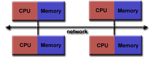
Nowadays, MPI runs on virtually any hardware platform.
Running MPI
So how do we go about running MPI in Python? Thankfully is it a simpler process than C or Fortran, as we normally need
an MPI call to start the MPI library. In Python, this isn’t needed as importing the mpi4py library is enough.
from mpi4py import MPI
The MPI program is launched as a set of independent, identical processes. These execute the same program code and
instructions, and can reside on different nodes/computers. There are a number of different ways to launch MPI programs,
and these differ based on whatever system you are running on differs depending on the system. Examples include, but are
not limited to mpirun, mpiexec, srun
Important to note while using MPI
MPI is not best utilised in a Jupyter notebook environment. This is because they are best used for demonstations and testing. If you wish to implement
mpi4pyin a working environment, we highly recommend you do so outside of a notebook environment.If you are running MPI on an HPC system, you MUST NOT USE THE LOGIN NODES. You should use compute nodes when running MPI code otherwise your jobs may be killed, you will restrict other users or worse be kicked out of the HPC!
Before we get to submitting files etc, we need to discuss the main things one needs in an MPI program. The first of these is a communicator.
A communicator is a group of processes that contains all processes that will participate in communication. In mpi4py
most MPI calls are implemented as methods of a communicator object. This is done using MPI.COMM_WORLD. The user can
define custom communicators, which will be covered in a later section.
Once you have a communicator set up, you need a way of identifying all the MPI processes. These are known as ranks. A rank is a logical ID number given to a process, and can also be used as a way to query the rank. Because of this feature, processes can perform different tasks based on their rank. You will get the chance to write code that follows the following format.
if (rank == 0):
    # do something
elif (rank == 1):
    # do something else
else:
    # all other processes do something else
Aside from the rank, the number of processes also needs to be known. This is called the size, and is specified when you initiate the program, i.e. at runtime. After importing MPI, the beginning of any MPI program will have the following three instructions.
comm = MPI.COMM_WORLD
size = comm.Get_size()
rank = comm.Get_rank()
You will find that the most common routines in MPI include:
- Communication between processes, sending and receiving messages between 2 or more processes
- Synchronization between processes
- Communicator creation and manipulation
- Advanced features (e.g. user defined datatypes, one-sided communication and parallel I/O)
As one needs to submit MPI python files to compute nodes, it means that you will need to write a job script to submit to the queue. An example is shown below. MPI can technically work on login nodes, however you should always submit code with MPI to the queue.
#!/bin/bash
#SBATCH --nodes=1
#SBATCH --time=00:10:00
#SBATCH -A $ACCOUNT_NAME
#SBATCH --job-name=$JOB_NAME
#SBATCH -p $QUEUE_NAME
#SBATCH --reservation=$RESERVATION_NAME

module purge
module load conda
module list

source activate $ENVIRONMENT

cd $SLURM_SUBMIT_DIR

mpirun -np N python3 $FILE_TO_RUN

exit 0
As you can see, the python files are run a bit differently when utilising MPI, as we need to specify (here with
mpirun) that we want to utilise the MPI library. Next we have the notation -np N, where -np stands for
number of processes and N refers to the number of processes you wish to execute. For the purposes of this lesson,
and the exercises, we will specifically say how many processes to use.
“Hello World” in MPI
from mpi4py import MPI

# communicator containing all processes
comm = MPI.COMM_WORLD

size = comm.Get_size()
rank = comm.Get_rank()

print("I am rank %d in group of %d processes" % (rank, size))
In the job script (which we can call job.sh), we can use the following line to run MPI.
mpirun -np 4 python3 hello.py
$ sbatch job.sh
You will receive a job ID number, which can be used to query the job status or delete the job if needed. The expected output will be something similar to:
I am rank 0 in group of 4 processes
I am rank 1 in group of 4 processes
I am rank 2 in group of 4 processes
I am rank 3 in group of 4 processes
We say “similar to” as this output may not be replicated. The processes may finish at different times, so therefore you may get the outputs in a different order. It also serves as proof that it is not serialised (i.e. one process runs straight after another).
Running your first MPI program
Using the code below, set up the communicator, rank and size, and then create a list from 1-4, and use a for loop to multiply the element of the list by the rank. Add a print statement to show how the array changes depending on the rank.
Use the job script template as shown further above. Your instructor will give you the items to replace for the variables
$ACCOUNT_NAME,$QUEUE_NAMEand$RESERVATION_NAME. You can choose the$JOB_NAMEyourself.from mpi4py import MPI # TODO: Set up communicator # TODO: Get the rank # TODO: Get the size # TODO: Create array and loop print("I am rank %d in group of %d processes" % (rank, size)) # TODO: Add print statementSolution
from mpi4py import MPI

# communicator containing all processes
comm = MPI.COMM_WORLD

size = comm.Get_size()
rank = comm.Get_rank()

arr = [1,2,3,4]
for i in range(len(arr)):
    arr[i] = i*rank

print("I am rank %d in group of %d processes" % (rank, size))
print("My list is", arr)
Point to Point communication
Point to Point communication in its simplest terms is like a game of ping pong. Imagine the ping-pong ball as your
message, and each racket as a process. MPI does its communications through messages, and these, in computational terms
are a number of elements of a particular datatype. These can be basic or special MPI derived datatypes. Point to Point
communication itself is when a source (src) sends a message to a destination. But like with ping pong, if you
send/serve the ball/message you don’t just need both sides of the table. You need a destination, (dest) i.e. another
racket/process to receive it.
This communication takes place within the communicator MPI.COMM_WORLD. Each process in a communicator is identified
by their ranks in the communicator. Sends and receives in a program should match, one receive per send, like with our
ping pong rally.
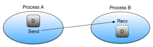
When it comes to sends and receives, there are two main types.
Synchronous Send: Imagine this situation like a WhatsApp message, you send the message, and you see a green tick appear showing that the message is sent, and another that it has been received (followed by them turning blue showing it has been read). This is known as a synchronous send, as you, the sender knows that the message has been received.
Buffered/Asynchronous Send: An asynchronous send is analogous to sending a message in the mail. You, the sender know that the message has left, but do not know whether it has been or will be received.
We will now move onto an example that uses send and receive, and we will run this with 4 ranks.
from mpi4py import MPI

# communicator containing all processes
comm = MPI.COMM_WORLD
rank = comm.Get_rank()

if rank == 0:
    data = {'a': 7, 'b': 3.14}
    comm.send(data, dest=1)
    print('rank ', rank, ' sent: ', data)
elif rank == 1:
    data = comm.recv(source=0)
    print('rank ', rank, ' received: ', data)
else:
    print('rank ', rank, ' did not receive data')
We set up our communicator, comm as well as our rank and use these objects to call send and recv as well as
querying and returning our ranks. We continue with our rank 0, which contains some data, in this case a dictionary, and
we want to send this data, to a destination, and we specify the destination rank. If you have used MPI with C and
Fortran this is a simplified notation.
Now, we want to say that if our rank equals 1, we have to receive it, for every send in this way of doing this we need
a receive, specifying the rank from which the message came from. If we are at rank=0 and rank=1 sent a message, we
need to know to expect a message from rank=1. If, however, we are told to expect a message instead from rank=2, we
will be waiting until the end of time for that message to arrive. A message that was never sent. These are known as
deadlocks and we will cover them in more detail in the
next episode. For now
though let us look at our output.
rank  3  did not receive data
rank  2  did not receive data
rank  0  sent:  {'a': 7, 'b': 3.14}
rank  1  received:  {'a': 7, 'b': 3.14}
As we can see in our output, ranks 2 and 3 did not receive any data, because we never specified the tasks for these processes to do. Technically they did, issuing a print statement, but no more than that. Prior to sending the data, rank 1 was empty, and now, having received the data, from rank 0, the latter is now empty. The data is provided as a return value in rank 1.
Typical Point-to-Point communication patterns include pariwise exchanges, where processes talk to their neighbours. The incorrect ordering of sends and receives can result in a deadlock.
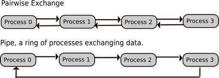
Pairwise exchange
Copy the code block below into a file caled
pairwise_exchange.py, implement a one-dimensional pairwise exchange of the ranks ofNprocesses with periodic boundary conditions. That is, each process communicates its rank to each of its topological neighbours.from mpi4py import MPI comm = MPI.COMM_WORLD rank = comm.Get_rank() size = comm.Get_size() # TODO: Define neighbours # TODO: Use send and recv to set up neighbours print ('I am process ', rank, ', my neighbours are processes', left, ' and ', right)For 4 processes, the output will be similar to;
I am process  1 , my neighbours are processes 0  and  2
I am process  3 , my neighbours are processes 2  and  0
I am process  0 , my neighbours are processes 3  and  1
I am process  2 , my neighbours are processes 1  and  3
HINT: left_rank is related to the rank and the size, but how? If you are a rank, what would you perceive as being left and right? You will need multiple sends and receives
Solution
from mpi4py import MPI

comm = MPI.COMM_WORLD
rank = comm.Get_rank()
size = comm.Get_size()

left_rank = (rank - 1) % size
right_rank = (rank + 1) % size

if (rank % 2) == 0:
    comm.send(rank, dest=right_rank)
    comm.send(rank, dest=left_rank)
    left = comm.recv(source=left_rank)
    right = comm.recv(source=right_rank)
else:
    left = comm.recv(source=left_rank)
    right = comm.recv(source=right_rank)
    comm.send(rank, dest=right_rank)
    comm.send(rank, dest=left_rank)

print ('I am process ', rank, ', my neighbours are processes', left, ' and ', right)
Case Study Parallel sum
Let us walk through a parallel sum case study. The idea is that we scatter our data between two processes, P0 and P1. Half of our array is sent to P1, and from there P0 and P1 independently sum their segments. From there, the summed array needs to be reduced, i.e. put back together again, from which P0 then sums the partial sums.

Step 1.1: Receive operation in scatter
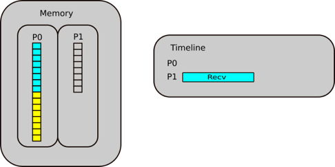
P1 posts a receive to receive half of the array FROM P0
Step 1.2: Send operation in scatter
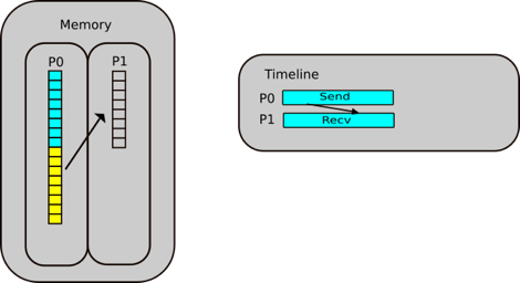
P0 posts a send to send the lower half of the array TO P1
Step 2: Compute the sum in parallel
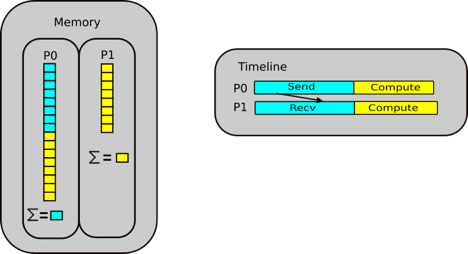
P0 & P1 compute their parallel sums and stores them locally
Step 3.1: Receive operation in reduction

P0 posts a receive to receive the partial sum
Step 3.2: Send operation in reduction

P1 posts a send to send partial sum
Step 4: Compute the final answer.
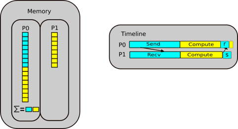
P0 sums the partial sums
Parallel sum implementation
Implement the parallel sum case study. That is;
- take the code block below
- implement the appropriate send/receive to distribute the data from rank 0
- perform the partial sum on each process
- implement the appropriate send/receive to gather the data at rank 0
- compute the final sum from the gathered data on rank 0
(Bonus) For added difficulty (and best practice), try to implement the same approach with an arbitrary number of processes.
from mpi4py import MPI
import numpy as np

comm = MPI.COMM_WORLD
rank = comm.Get_rank()

local_data = np.empty( , dtype=int)

# Distribute data
if rank==0:
    data = np.arange(100, dtype=int)
    local_data = data[] # TODO: choose appropriate range
    # TODO: Communicate
else:
    # TODO: Communicate

# TODO: Compute local and partial sums
local_sum = np.sum(local_data)

# Collect data
if rank==0:
    partial_sums = np.empty( , dtype=int)
    # TODO: Communicate

    # TODO: Calculate total sum

    # TODO: Print result
else:
    # TODO: Communicate
Solution
from mpi4py import MPI
import numpy as np

comm = MPI.COMM_WORLD
rank = comm.Get_rank()
size = comm.Get_size()

n = 100
local_n = n // size

local_data = np.empty(local_n , dtype=int)

# distribute data
if rank==0:
    data = np.arange(100, dtype=int)
    local_data = data[:local_n] # choose appropriate range

    # communicate
    for i in range(1, size):
        comm.Send(data[i*local_n:(i + 1)*local_n], i)
else:
    comm.Recv(local_data, 0)
Communicating arrays
Now we move onto communicating numpy arrays, and this is where you need to be careful. There are two sends and receives
in mpi4py, send/Send and recv/Recv. As you can see one is capitalised, the other is not. It is important to
point out that data needs to exist in the receive buffer, whereas for items like a dictionary all we needed to say is
that there is data coming from another rank. In the example below So here we are sending an array of floats of
size=10, and we need a buffer, we call the variable data to receive that array into. It works a bit like sending
apples from one basket into another. The receive cannot happen if there is no “basket” to put it into.
from mpi4py import MPI
import numpy as np

comm = MPI.COMM_WORLD
rank = comm.Get_rank()

if rank==0:
    data = np.arange(10, dtype=float)
    comm.Send(data, dest=1)
    print('rank ', rank, ' sent: ', data)
elif rank==1:
    data = np.empty(10, dtype=float)
    comm.Recv(data, source=0)
    print('rank ', rank, ' received: ', data)
Running the code will provide the following output.
rank  0  sent:  [0. 1. 2. 3. 4. 5. 6. 7. 8. 9.]
rank  1  received:  [0. 1. 2. 3. 4. 5. 6. 7. 8. 9.]
Combined Send and Receive
This is a fairly simple concept which combines the two commands send and recv into a single command. We will use
what we learned in the previouus section to use NumPy arrays.
from mpi4py import MPI
import numpy as np

comm = MPI.COMM_WORLD
rank = comm.Get_rank()

# Send buffer
data = np.arange(10, dtype=float) * (rank + 1)

# Receive buffer
buffer = np.empty(10, float)

if rank==0:
    dest, source = 1, 1
elif rank==1:
    dest, source = 0, 0

print('rank ', rank, ' send buffer: ', data)

comm.Sendrecv(data, dest=dest, recvbuf=buffer, source=source)

print('rank ', rank, ' receive buffer: ', buffer)
Running this code with 2 processes produces the following output.
rank  0  send buffer:  [0. 1. 2. 3. 4. 5. 6. 7. 8. 9.]
rank  0  receive buffer:  [ 0.  2.  4.  6.  8. 10. 12. 14. 16. 18.]
rank  1  send buffer:  [ 0.  2.  4.  6.  8. 10. 12. 14. 16. 18.]
rank  1  receive buffer:  [0. 1. 2. 3. 4. 5. 6. 7. 8. 9.]
Now that you have a clear idea of the power of a combined send and receive, let us now modify our pairwise code.
SendRecv pairwise exchange
Modify the pairwise exchange code from Exercise 2 to use the combined send/recv communication.
Solution
from mpi4py import MPI

comm = MPI.COMM_WORLD
rank = comm.Get_rank()
size = comm.Get_size()

left_rank = (rank - 1) % size
right_rank = (rank + 1) % size

right = comm.sendrecv(rank, dest=right_rank, source=left_rank)
left = comm.sendrecv(rank, dest=left_rank, source=right_rank)

print ('I am process ', rank, ', my neighbours are processes', left, ' and ', right)
Key Points
MPI is the true way to achieve parallelism
mpi4pyis an unofficial library that can be used to implement MPI in PythonA communicator is a group containing all the processes that will participate in communication
A rank is a logical ID number given to a process, and therefore a way to query the rank
Point to Point communication is the communication between two processes, where a source sends a message to a destination process which has to then receive it
Non-blocking and collective communications
Overview
Teaching: 60 min
Exercises: 30 minQuestions
Why do we need non-blocking communication?
What are the different collective routines and how can I implement them?
Objectives
Understand the difference between blocking and non-blocking communication
Implement different collective routines
![]()
Non-blocking communication
In the previous episode we covered the basics of MPI, becoming familiar with communicators, rank, size, and running MPI
for simple calculations and then onto sending and receiving. It’s all well and good but the communication types we
covered introduce the risk of deadlocks. These can similar to infinite loops or more specifically have a
situation where one process is expecting a message, but it was never even sent. These deadlocks will continue until
the program is physically terminated. This can be resolved with non-blocking communication. The routines covered so far,
send, Send, recv and Recv are all blocking routines. Let us walk through a common scenario of a cyclic structure.

In this example, all our processes form part of a ring, with rank 0’s neighbours being rank 1 and rank 3, and so on. We also have a non cyclic workflow.

If we try and program this with MPI Send and Recv, it can be dangerous. If we have small messages this is can work,
but as soon as the programmer ends up dealing with larger messages, they can become unstuck. MPI has a synchronous
protocol, and as soon as this switch happens, all the processes stop in MPI Send, meaning that Recv is never called
which means that all the processes will be blocked forever.
For non-cyclic workflows, there is an upside, as the last process is not calling Send, so this will start Recv, then the next rank will start receive, so we have a serialisation routine.
Which is better?
Which is a better situation to end up in? Having a;
- Serialised routine?
OR
- A deadlock?
Solution
Contrary to what you may think, a deadlock is better in this circumstance, because you can easily identify it and then promptly fix it. The non-cyclic situation is worse, as you have no indication that your code is being slowed down by a factor of 3.
Imagine if you had 10 processes, 50, 100? What if you have 1000 processes in 3 dimensions, 9 connections between them. Think about how much slowdown there would be if it was a serialised code! Something which in your mind that should take 10 minutes may take 10 hours, or more!
To work with non-blocking communication our workflow can be split into 3 phases.
rank = comm.Get_rank()
size = comm.Get_size()

if rank == 0:
    data = np.arange(size, dtype=float) * (rank + 1)
    # start a send
    req = comm.Isend(data, dest=1)
    # ... do something else ...
    calculate_something(rank)
    # wait for the send to finish
    req.wait()
    # now safe to read/write data again

elif rank == 1:
    data = np.empty(size, dtype=float)
    # post a receive
    req = comm.Irecv(data, source=0)
    # ... do something else ...
    calculate_something(rank)
    # wait for the receive to finish
    req.wait()
    # data is not ready to use
-
Initiate nonblocking communication. This returns immediately and sends/receives in the background. Our return value is set up as a request object The notation for non-blocking send is
Isend, and for receive,Irecv. ThisIstands for “incomplete” or “immediate” and are done locally, returning independently of any other processes activity. -
Do some work, be it related to what you want done in the process or some other communication. The most important usage area is to overlap communication with other communication. Or indeed you could have several communicators that use the MPI library in parallel.
-
From there, we wait for nonblocking communication to complete. The send buffer is read out of recv is readlly read in.
In summary, like an email you send it, then you can do other work until you hear a noise informing you that your email
has been sent, at which point your send buffer is refreshed. From there, call Irecv, and do some work, wait until
the message has arrived. Let’s think again of our example working with a ring.
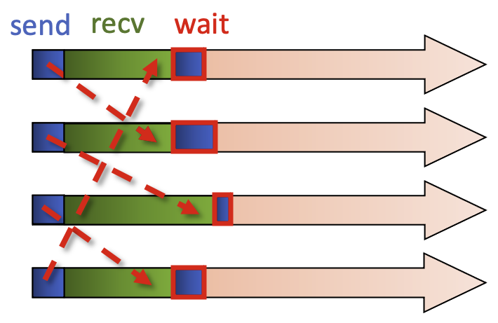
We call the non-blocking sends and these come back immediately, and from there we can call the blocking recv, so all
processes are calling the blocking recv. Now we have a non-blocking send and a blocking recv. This then allows the
message to flow. We then call the MPI command to wait for the non-blocking send. Because the message has been
received there is no need for extra waiting, and then you can reuse the send buffer.
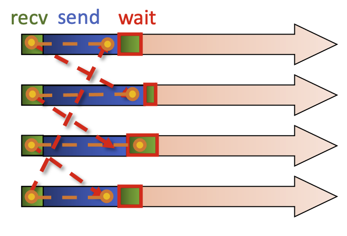
The alternative is to initiate a non-blocking receive, with each process calling receive. The other work we can do is a blocking send, the message can be transferred.
Here is another example, where one needs to know the boundary conditions in a process. In P0, we have our final row,
the border_data and then some ghost_data as well as the local_data that stays local to the process, in this case
P0.
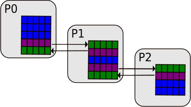
request = comm.Irecv(ghost_data)
request2 = comm.Isend(border_data)
compute(ghost_independent_data)
request.wait()
compute(border_data)
We initialise a request to Irecv (or receive in a non-blocking way) the ghost_data from process 1, and then use the
non-blocking Isend on the border_data to process 1 so it can then do its own calculation. We can then continue and
do some other work, as it is non-blocking. This is represented by a generic function which operates on
ghost_independent_data then wait for the sending and receiving to complete, and then we can work on the border data.
We need to briefly touch on “waiting” for data. When it comes to dealing with multiple non-blocking operations,
waitany() and waitall() methods can be very helpful, and are available in the MPI.Request class.
Let us now look at a working example with a small array before our next challenge. Note the import of the Request
class ou can have a little go of this yourselves. Note that we import the Request class while we import the other
items we need.
from mpi4py import MPI
from mpi4py.MPI import Request
import numpy as np

comm = MPI.COMM_WORLD
rank = comm.Get_rank()

# data = send buffer
data = np.arange(10, dtype=float) * (rank + 1)
# buffer = receive buffer
buffer = np.zeros(10, dtype=float)

print('rank', rank, 'sending:', data)

if rank == 0:
    req = [comm.Isend(data, dest=1)]
    req.append(comm.Irecv(buffer, source=1))
if rank == 1:
    req = [comm.Isend(data, dest=0)]
    req.append(comm.Irecv(buffer, source=0))

print('rank', rank, 'receive buffer before wait:', buffer)

Request.waitall(req)
We set up our data which is a simple size=10 numpy array multiplied by the (rank + 1), and our receive buffer, where this will be put into. These now will exist in both rank 0 and 1.
On output with 2 processes you should expect the following result.
rank 0 sending: [0. 1. 2. 3. 4. 5. 6. 7. 8. 9.]
rank 0 receive buffer before wait: [0. 0. 0. 0. 0. 0. 0. 0. 0. 0.]
rank 0 receive buffer after wait: [ 0.  2.  4.  6.  8. 10. 12. 14. 16. 18.]
rank 1 sending: [ 0.  2.  4.  6.  8. 10. 12. 14. 16. 18.]
rank 1 receive buffer before wait: [0. 0. 0. 0. 0. 0. 0. 0. 0. 0.]
rank 1 receive buffer after wait: [0. 1. 2. 3. 4. 5. 6. 7. 8. 9.]
So, when it comes to point-to-point communication, non-blocking communication is often the best method to go to with the aim of reducing the probability of deadlocks. This is the most important concept of MPI, and we recommend spending a good bit of time trying to wrap your head around it! Once you are comfortable with it, you are well set for most other problems you may encounter.
Non-blocking communication in a ring
Before starting, it is important to state that this code can work, but it is still wrong, deceptively so as we have learned. Using a synchronous send,
Ssend, will definitely cause a deadlock. This example will run very quickly so if a result doesn’t come back in a matter of seconds, you have a deadlock. Using a regularSendwill at some point cause a deadlock, but not 100% of the time.The code is set up in such a way so that:
- A set of processes are arranged in a ring
- Each process stores its rank in MPI.COMM_WORLD into an integer variable, snd_buf
- Each process passes this snd_buf to the neighbour on its right
- Prepares for the next iteration
- Each processor calculates the sum of all values Steps 2-4 are repeated with n number of times (number of processes) and each process calculates the sum of all ranks.
For this exercise only use
Issend, which is used to demonstrate a deadlock is the non-blocking routine is incorrectly used. Real applications useIsend, notIssend.You can monitor the status of your job with
squeue jobid. If you encounter a deadlock, you must cancel the job. Usescancel jobidto do so.from mpi4py import MPI import numpy as np rcv_buf = np.empty((), dtype=np.intc) #rcv_buf = np.empty((), dtype=np.intc) # uninitialized 0 dimensional integer array status = MPI.Status() comm = MPI.COMM_WORLD my_rank = comm.Get_rank() size = comm.Get_size() right = (my_rank+1) % size left = (my_rank-1+size) % size sum = 0 snd_buf = np.array(my_rank, dtype=np.intc) # 0 dimensional integer array with 1 element initialized with the value of my_rank for i in range(size): comm.Send((snd_buf, 1, MPI.INT), dest=right, tag=17) #request = comm.Isend((snd_buf, 1, MPI.INT), dest=right, tag=17) comm.Recv((rcv_buf, 1, MPI.INT), source=left, tag=17, status=status) #request.Wait(status) np.copyto(snd_buf, rcv_buf) # We make a copy here. What happens if we write snd_buf = rcv_buf instead? sum += rcv_buf print(f"PE{my_rank}:\tSum = {sum}")Solution
from mpi4py import MPI
import numpy as np

rcv_buf = np.empty((), dtype=np.intc)
status = MPI.Status()

comm = MPI.COMM_WORLD
my_rank = comm.Get_rank()
size = comm.Get_size()

right = (my_rank+1) % size
left  = (my_rank-1+size) % size

sum = 0
snd_buf = np.array(my_rank, dtype=np.intc) # 0-D integer array with 1 element initialized with the value of my_rank

for i in range(size):
   # Official solution to be used in your code outside of lesson
   request = comm.Isend((snd_buf, 1, MPI.INT), dest=right, tag=17)
   comm.Recv((rcv_buf, 1, MPI.INT), source=left,  tag=17, status=status)
   request.Wait(status)
   np.copyto(snd_buf, rcv_buf)
   sum += rcv_buf
print(f"PE{my_rank}:\tSum = {sum}")
Collective communication
Collective communication is the step up from simple sends and receives, as it transmits data among all processes in a process group. Regardless of what process group you are in (more on communicator groups later), these routines must be called by all processes in a given group, so you need to be careful about having the correct amount of sent and received data.
These operations can be used for data movement, collective computation or synchronization. The idea of collective communication is to shorten the material we had in our send receive codes into a single line.
Broadcasting
With broadcasting (Bcast), an array on rank 0 can be communicated to all other tasks. The data is not modified in any
way and all the processes receive the same data.
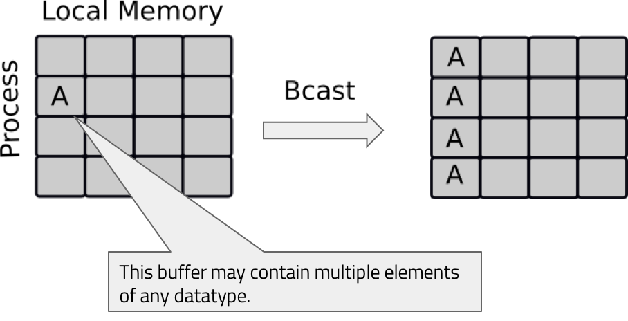
Let’s looks at a broadcasting code. We have our communicator, and rank, and we are broadcasting a python dictionary and a NumPy array to all the other processes. As with sends and receives, we have an upper and lowercase broadcast, so all the other processes aside from rank 0 have empty NumPy arrays of the same size. For the python object it doesn’t matter, but you do need to declare that the variable actually exists.
from mpi4py import MPI
import numpy as np

comm = MPI.COMM_WORLD
rank = comm.Get_rank()

if rank == 0:
    # Python object
    py_data = {'key1' : 0.0, 'key2' : 11}
    # NumPy array
    data = np.arange(8)/10
else:
    py_data = None
    data = np.zeros(8)

# Broadcasting the python object
new_data = comm.bcast(py_data, root=0)
print('rank', rank, 'received python object:', new_data)
# Broadcasting the NumPy array
comm.Bcast(data, root=0)
print('rank', rank, 'received NumPy array:', data)
Upon running this with 4 processes you should expect the following output.
rank 0 received python object: {'key1': 0.0, 'key2': 11}
rank 0 received NumPy array: [0.  0.1 0.2 0.3 0.4 0.5 0.6 0.7]
rank 1 received python object: {'key1': 0.0, 'key2': 11}
rank 1 received NumPy array: [0.  0.1 0.2 0.3 0.4 0.5 0.6 0.7]
rank 2 received python object: {'key1': 0.0, 'key2': 11}
rank 2 received NumPy array: [0.  0.1 0.2 0.3 0.4 0.5 0.6 0.7]
rank 3 received python object: {'key1': 0.0, 'key2': 11}
rank 3 received NumPy array: [0.  0.1 0.2 0.3 0.4 0.5 0.6 0.7]
Next we will look at scattering.
Scattering

Scattering is very similar to broadcasting, but the difference is important. MPI Broadcast, like the news sends the same information to all processes, whereas Scatter sends chunks of an array to different processes.
If you have watched BBC news, you have the main broadcast, think of like MPI Bcast, followed up intermittently by the regional information, one for Northern Ireland, one for Midlands, Scotland etc. That is similar to a scatter.
Looking at an example, for our lowercase scatter, we only need our python data and the root process, however for the NumPy scatter, we need a receive buffer.
from mpi4py import MPI
import numpy as np

comm = MPI.COMM_WORLD
rank = comm.Get_rank()
size = comm.Get_size()

if rank == 0:
    # Python object
    py_data = range(size)
    data = np.arange(size**2, dtype=float)
else:
    py_data = None
    data = None
print("Original data = ", data)

# Scatter the python object
new_data = comm.scatter(py_data, root=0)
print('rank', rank, 'received python object:', new_data)

# Scatter the NumPy array
# A receive buffer is needed here!
buffer = np.empty(size, dtype=float)
comm.Scatter(data, buffer, root=0)
print('rank', rank, 'received NumPy array:', buffer)
Upon running this with 4 processes you should expect the following output.
Original data =  [ 0.  1.  2.  3.  4.  5.  6.  7.  8.  9. 10. 11. 12. 13. 14. 15.]
rank 0 received python object: 0
rank 0 received NumPy array: [0. 1. 2. 3.]
Original data =  None
rank 2 received python object: 2
rank 2 received NumPy array: [ 8.  9. 10. 11.]
Original data =  None
rank 3 received python object: 3
rank 3 received NumPy array: [12. 13. 14. 15.]
Original data =  None
rank 1 received python object: 1
rank 1 received NumPy array: [4. 5. 6. 7.]
Gathering

Gathering is the inverse of Scatter. Instead of spreading elements from one process to many processes, MPI_Gather takes elements from many processes and gathers them to one single process. This routine is highly useful to many parallel algorithms, such as parallel sorting and searching.
Using the combination of Scatter and Gather you can do a lot of useful things, a very simple example being the computation of the average of numbers.
For the demonstration we want an list n that gets the gathered ranks, this is a simple python list. As with Scatter, Gather needs a buffer which we define here.
So as you can see these three have a lot in common and behave similarly.
from mpi4py import MPI
import numpy as np

comm = MPI.COMM_WORLD
rank = comm.Get_rank()
size = comm.Get_size()

data = np.arange(10, dtype=float) * (rank + 1)

# Gather the value of rank from each rank, then send to rank 0
n = comm.gather(rank, root=0)

# Gather the NumPy array from each rank, then send to rank 0
buffer = np.zeros(size * 10, dtype=float)
comm.Gather(data, buffer, root=0)

if rank == 0:
    print('gathered ranks:', n)
    print('gathered NumPy arrays:', buffer)
Upon running this with 4 processes you should expect the following output.
gathered ranks: [0, 1, 2, 3]
gathered NumPy arrays: [ 0.  1.  2.  3.  4.  5.  6.  7.  8.  9.  0.  2.  4.  6.  8. 10. 12. 14.
 16. 18.  0.  3.  6.  9. 12. 15. 18. 21. 24. 27.  0.  4.  8. 12. 16. 20.
 24. 28. 32. 36.]
Point to Point –> Gather
The Send and Receive code here works perfectly as is, but using
gatherwould certainly make things much cleaner, as we only have to call one MPI command.Substitute the point-to-point communication with one call to
gather. Watch out to ensurefrom mpi4py import MPI import numpy as np comm = MPI.COMM_WORLD my_rank = comm.Get_rank() num_procs = comm.Get_size() # Each process assigned some work res = np.array(my_rank**2, dtype=np.double) print(f"I am process {my_rank} out of {num_procs}, result={res:f}") if (my_rank == 0): res_arr = np.empty(num_procs, dtype=np.double) # TODO: Substitute the following block with MPI_Gather ### if (my_rank != 0): # Sending some results from all processes (except 0) to process 0: comm.Send((res, 1, MPI.DOUBLE), dest=0, tag=99) else: res_arr[0] = res # process 0's own result # Receive all the messages for rank in range(1,num_procs): # Result of processes 1 -> n comm.Recv((res_arr[rank:], 1, MPI.DOUBLE), source=rank, tag=99, status=None) ### if (my_rank == 0): for rank in range(num_procs): print(f"I'm proc 0: result of process {rank} is {res_arr[rank]:f}")Solution
from mpi4py import MPI
import numpy as np

#MPI-related data
comm = MPI.COMM_WORLD
my_rank = comm.Get_rank()
num_procs = comm.Get_size()

result = np.array(my_rank**2, dtype=np.double)
print(f"I am process {my_rank} out of {num_procs}, result={result:f}")

if (my_rank == 0):
   res_arr = np.empty(num_procs, dtype=np.double)
else:
   res_arr = None

comm.Gather((result,1,MPI.DOUBLE), (res_arr,1,MPI.DOUBLE), root=0)
if (my_rank == 0):
   for rank in range(num_procs):
      print(f"I'm proc 0: result of process {rank} is {res_arr[rank]:f}")
Reduction Operation
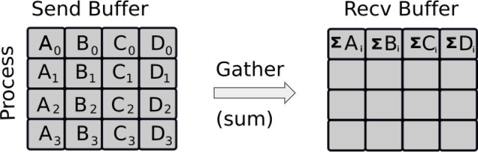
Reduce is a classic concept from functional programming. Data reduction involves reducing a set of numbers into a
smaller set of numbers via a function. For example, let’s say we have a list of numbers [1, 2, 3, 4, 5]. Reducing
this list of numbers with the sum function would produce sum([1, 2, 3, 4, 5]) = 15. Similarly, the multiplication
reduction would yield multiply([1, 2, 3, 4, 5]) = 120.
As you might have imagined, it can be very cumbersome to apply reduction functions across a set of distributed numbers.
Along with that, it is difficult to efficiently program non-commutative reductions, i.e. reductions that must occur in
a set order. Luckily, MPI has a handy function called MPI_Reduce that will handle almost all of the common reductions
that a programmer needs to do in a parallel application.
Calculating a reduction: primer
Below we will look at reduce routines for a single integer (rank) and a numpy array, which on each process is [0,1,2,3] * (rank + 1)
What would the rank reduction be? Similarly for the NumPy array?
Solution
The rank reduction is equal to 3.
The NumPy array on the other hand is calculated as follows:
[0,1,2,3]
[0,2,4,6]
[0,3,6,9]
=[0,6,12,18]
Let’s look at our example. We specify the type of reduction that we want as well as the root rank, the operation
op is optional, and defaults to MPI.SUM, which will return the sum. Alternatively you can use MPI.PROD for the
product. Feel free to check it out.
from mpi4py import MPI
import numpy as np

comm = MPI.COMM_WORLD
rank = comm.Get_rank()
size = comm.Get_size()

data = np.arange(10, dtype=float) * (rank + 1)
print(data)
# Gather the value of rank from each rank, then send to rank 0
n = comm.reduce(rank, root=0)

# Gather the NumPy array from each rank, then send to rank 0
buffer = np.zeros(10, dtype=float)
comm.Reduce(data, buffer, root=0)

if rank == 0:
    print('rank reduction:', n)
    print('NumPy reduction:', buffer)
Upon running this with 3 processes you should expect the following output.
[ 0.  3.  6.  9. 12. 15. 18. 21. 24. 27.]
[ 0.  2.  4.  6.  8. 10. 12. 14. 16. 18.]
[0. 1. 2. 3. 4. 5. 6. 7. 8. 9.]
rank reduction: 3
NumPy reduction: [ 0.  6. 12. 18. 24. 30. 36. 42. 48. 54.]
Global reduction
The communication around a ring earlier can be further simplified using a global reduction. Modify your solution by:
- Determining the quantity of code that needs to be replaced by the global reduction
- Using
Allreduceto call the collective reduction routineSolution
from mpi4py import MPI
import numpy as np

comm_world = MPI.COMM_WORLD
my_rank = comm_world.Get_rank()
size = comm_world.Get_size()

snd_buf = np.array(my_rank, dtype=np.intc)
sum = np.empty((), dtype=np.intc)

# Compute sum of all ranks.
comm_world.Allreduce(snd_buf, (sum,1,MPI.INT), op=MPI.SUM )
# Also possible
# comm_world.Allreduce((snd_buf,1,MPI.INT), (sum,1,MPI.INT), op=MPI.SUM)
# Shortest version in python is
# comm_world.Allreduce(snd_buf, sum)

print(f"PE{my_rank}:\tSum = {sum}")
Other Collective operations
Collectives are very common in MPI programming and there is a large array of commands that can be used, even in
mpi4py. It is important to remember that Python is not officially supported by MPI, so there is a chance that the
command you are looking for may not exist in mpi4py. Non-blocking collectives are a prime example of this. These
enable the overlapping of communication and computation together with the benedits of collective communication, but:
- They have to be called in same order by all ranks in a communicator
- The mixing of blocking and non-blocking collectives is not allowed
In any case, these types of routines can only be used in C and Fortran.
Despite this, there are a few other common collective operations which can be utilised in mpi4py.
Scatterv:- Each process receives different amount of data.Gatherv: Each process sends different amount of data.Allreduce: All processes receive the results of reduction.Alltoall: Each process sends and receives to/from each otherAlltoallv: Each process sends and receives different amount of data to/from each other
There can be problems with collectives however!
- Using a collective operation within one branch of an if-test of the rank. Remember, all processes in a communicator must call a collective routine
if rank == 0: comm.bcast(...)
- Assuming that all processes making a collective call would complete at the same time.
- Using the input buffer as the output buffer:
comm.Scatter(a, a, MPI.SUM)
An easier look at collectives
Head to the Jupyter notebook here and scroll down to Easier Exercise: Collective Communication, and work on an easier script that utilises
Broadcast,Scatter,Gather, andReduce.Solution
Full solution can be found here
Communicators
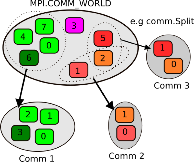
So far we have been dealing with a single communicator, MPI_COMM_WORLD. All processes that we want to involve in the
communication, are part of that communicator, however we can split up the processes to work in different communicators
so they do different things. Like a coupled weather model. MPI_COMM_WORLD works on the communication of the entire
program, then within it you can have a communicator called EARTH, which will undertake work on the Earth system,
ATMOSPHERE for work on the atmosphere and so on.
We can split up these communicators as shown here. We have 8 ranks in MPI_COMM_WORLD, but as you can see in the
diagram above, as they go into the new communicators, their ranks reset from 0.
Let’s look at an example.
from mpi4py import MPI
import numpy as np

from mpi4py import MPI
comm = MPI.COMM_WORLD
rank = comm.Get_rank()

color = rank % 4

local_comm = comm.Split(color)
local_rank = local_comm.Get_rank()

print("Global rank: %d Local rank: %d" % (rank, local_rank))
Looking at the code you see we introduce a variable called color. The value determining in which group the calling
MPI process will be, MPI processes providing the same color value will be put in the same subgroup.
Global rank: 0 Local rank: 0
Global rank: 2 Local rank: 0
Global rank: 3 Local rank: 0
Global rank: 4 Local rank: 1
Global rank: 5 Local rank: 1
Global rank: 1 Local rank: 0
Global rank: 6 Local rank: 1
Global rank: 7 Local rank: 1
Looking at the output for 8 processes, we have defined two sub communicators, each with their own local ranks.
More communicators
Modify the Allreduce program from the previous exercise. You will need to split the communicator
MPI_COMM_WORLDinto 1/3 and 2/3, so the color variable for the input forSplitis;color = (rank > [$\frac{size -1}{3}$])
- Calculate sumA and sumB over all processes within each sub-communicator
- Run with 12 processes to produce the following results:
- sumA: Sums up ranks in MPI_COMM_WORLD: 4 & 8 split with world ranks;
- 0 -> 3 = 6
- 4 -> 11 = 60
- sumB: Sums up ranks within new sub-communicators: 4 & 8 split with sub-comm ranks:
- 0 -> 3 = 6
- 0 -> 7 = 28
sumA = np.empty((), dtype=np.intc)
sumB = np.empty((), dtype=np.intc)

comm = MPI.COMM_WORLD
size = comm.Get_size()
rank = np.array(comm.Get_rank(), dtype=np.intc)

# TODO
# 1. Define 'color' variable
# 2. Define your sub-communicator using a split
# 3. Define your new size and ranks
# 4. Keep track of your variable names for clarity

# Compute sum of all ranks.
comm.Allreduce(rank, (sumA, 1, MPI.INT), MPI.SUM)
comm.Allreduce(rank, (sumB, 1, MPI.INT), MPI.SUM)

print("PE world:{:3d}, color={:d} sub:{:3d}, SumA={:3d}, SumB={:3d} in comm_world".format(
          rank, "TODO: color", "TODO: sub_rank", sumA, sumB))
Solution
from mpi4py import MPI
import numpy as np

sumA = np.empty((), dtype=np.intc)
sumB = np.empty((), dtype=np.intc)

comm_world = MPI.COMM_WORLD
world_size = comm_world.Get_size()
my_world_rank = np.array(comm_world.Get_rank(), dtype=np.intc)

mycolor = (my_world_rank > (world_size-1)//3)
# This definition of mycolor implies that the first color is 0
sub_comm = comm_world.Split(mycolor, 0)
sub_size = sub_comm.Get_size()
my_sub_rank = np.array(sub_comm.Get_rank(), dtype=np.intc)

# Compute sum of all ranks.
sub_comm.Allreduce(my_world_rank, (sumA, 1, MPI.INT), MPI.SUM)
sub_comm.Allreduce(my_sub_rank,   (sumB, 1, MPI.INT), MPI.SUM)

print("PE world:{:3d}, color={:d} sub:{:3d}, SumA={:3d}, SumB={:3d} in sub_comm".format(
          my_world_rank, mycolor, my_sub_rank, sumA, sumB))
Key Points
In some cases, serialisation is worse than a deadlock, as you don’t know the code is inhibited by poor performance
Collective communication transmits data among all processes in a communicator, and must be called by all processes in a group
MPI is best used in C and Fortran, as in Python some function calls are either not present or are inhibited by poor performance
Dask
Overview
Teaching: 60 min
Exercises: 30 minQuestions
What is Dask?
How can I implement Dask array?
How can I use Dask MPI
Objectives
Implement Dask array
Implement Dask MPI
![]()
Dask
Dask is a framework that covers many things which were not possible even a few years ago. It allows us to create
multiple tasks with a minimum of effort. There are different aspects to Dask of which we will cover just a few during
this lesson. Dask is integrated with different projects such as pandas, numpy and scipy. This allows
parallelisation of for example scipy functions with minimum changes to the python code. Some of the projects have
their own multithreaded functions, so Dask is not essential.
Dask can work very well in notebook environments, as it gives you a good visual representation as to what is going on. You can open up the notebook for this episode.
We will first look at “Dask Distributed”. The first step is to create a set of workers with a scheduler. Here we are creating 2 “worker” processes with 2 threads each. This means that we can assign a particular task to a specific worker. There will be 1GB for all workers.
import dask
from dask.distributed import Client

client = Client(n_workers=2, threads_per_worker=2, memory_limit='1GB')

client
The Client function is needed here to set up a variable which we will call lowercase client. It is worth noting
that this is running on a login node, hence the memory size is small as we do not want to stress the system. As you can
see upon running the cell with (using the correct environment) your output will be very different to what you may
expect.
It will display some information about:
Client:
- Connection Method
- Cluster type
- Dashboard
And in the dropdown menu on Cluster Info: Local Cluster
- Dashboard
http://127.0.0.1:12345/status - Total threads: 4
- Status: running
- Workers: 2
- Total memory: 1.86 GiB
- Using processes: True
And in the second drop down menu about the scheduler Scheduler
- Comm:
... - Dashboard:
http://127.0.0.1:12345/status - Started: just now
- Workers: 2
- Total threads: 4
- Total memory: 1.86 GiB
Further information is then displayed about the two workers. This information is not essential, but can help you understand what is being set up.
Clicking the link in Dashboard will not work on its own. To deal with this you would need to set up an ssh tunnel through the machine that you are using the terminal.
$ ssh -N -L 8787:localhost:12345 youraccount@login1@kay.ichec.ie
You may be using Jupyter notebook already, which will be taking up the port 8080, so we can change that in the
terminal to 8787 as shown above. The second thing to change is the port that is being used on your host/machine. If
you look up at the Dashboard link, the final 5 numbers will show the port, in this case 12345. Yours may show up
differently.
Upon entering the required passwords, your tunnel is set up and you can view your Dashboard. Entering localhost:8787
into your web browser will produce something similar to below.
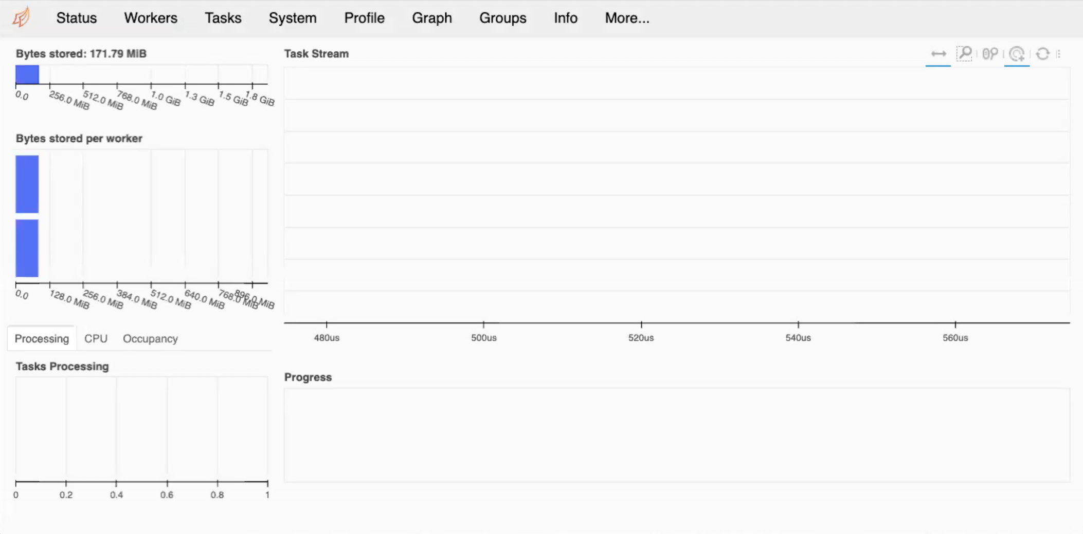
If you are doing debugging of your system and seeing what is going on with load balancing, then this can be very useful, giving you the amount of memory per worker and so on. If your program exceeds the memory usage specified in the code, then naturally, you will get some errors.
Dask Dashboard
Ensure that you have followed the above steps and take some time to explore around the Dashboard. What do you think everything means, and how can you best utilise them?
The alternative to the above method is to install jupyter-server-proxy.
Once we are finished with this we need to close the client, and therefore you will stop the workers.
client.close()
Using this type of cluster will however restrict you to a single node of your machine. We can use more than one node later on.
Here we have a simple example where we estimate pi. This version uses numpy functions to perform the calculations. Note there are no explicit loops. The code is serial. We are instead setting up an array, setting it up where we are asked for the size of array that we want to use. As the array gets bigger, our estiamte of pi will improve. As we are using NumPy to make it more efficient, we don’t necessarily need any loops.
import numpy as np

def calculate_pi(size_in_bytes):

    """Calculate pi using a Monte Carlo method."""

    rand_array_shape = (int(size_in_bytes / 8 / 2), 2)

    # 2D random array with positions (x, y)
    xy = np.random.uniform(low=0.0, high=1.0, size=rand_array_shape)

    # check if position (x, y) is in unit circle
    xy_inside_circle = (xy ** 2).sum(axis=1) < 1

    # pi is the fraction of points in circle x 4
    pi = 4 * xy_inside_circle.sum() / xy_inside_circle.size

    print(f"\nfrom {xy.nbytes / 1e9} GB randomly chosen positions")
    print(f"   pi estimate: {pi}")
    print(f"   pi error: {abs(pi - np.pi)}\n")

    return pi
%time calculate_pi(10000)
from 1e-05 GB randomly chosen positions
   pi estimate: 3.072
   pi error: 0.06959265358979305

CPU times: user 2.06 ms, sys: 1.44 ms, total: 3.5ms
Wall time: 2.78 ms

3.072
Without needing to change the function we can use Dask to parallelise the work. In this case we have two workers. The
dask.delayed creates a task graph, which creates the tasks that have to be run, if there are more than 2, they need
to be set to run using the scheduler until all tasks are complete. This doesn’t run the task itself however.
The running of the tasks itself is done using dask.compute
client = Client(n_workers=2, threads_per_worker=2, memory_limit='1GB')
dask_calpi = dask.delayed(calculate_pi)(10000)
Runtime with Dask
Check the output of the line below.
%time dask.compute(dask_calpi)Is this what you would expect? Why?
Result
CPU times: user 195 ms, sys: 343 ms, total: 538 ms
Wall time: 546 ms
(3.1488,)
You should find that it is taking longer with Dask! You can change the size of the problem but still find that Dask is slower. This is because we are using Dask incorrectly, the function cannot be divided into tasks. There are also a lot of overheads, which can still slow things down more.
We can visualise how the tasks are decomposed with the visualize function.
dask.visualize(dask_calpi)
You will get an output similar to below, which shows we are only using 1 task. We need to split our workload into multiple tasks.
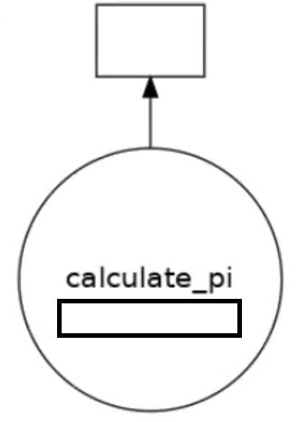
We can only get task parallelism if we call the function more than once. Below is an example of this.
results = []
for i in range(5):
    dask_calpi = dask.delayed(calculate_pi)(10000*(i+1))
    results.append(dask_calpi)

dask.visualize(results)

#to run all the tasks use
#dask.compute(*results)
Running this will produce the following output, now with 5 tasks.
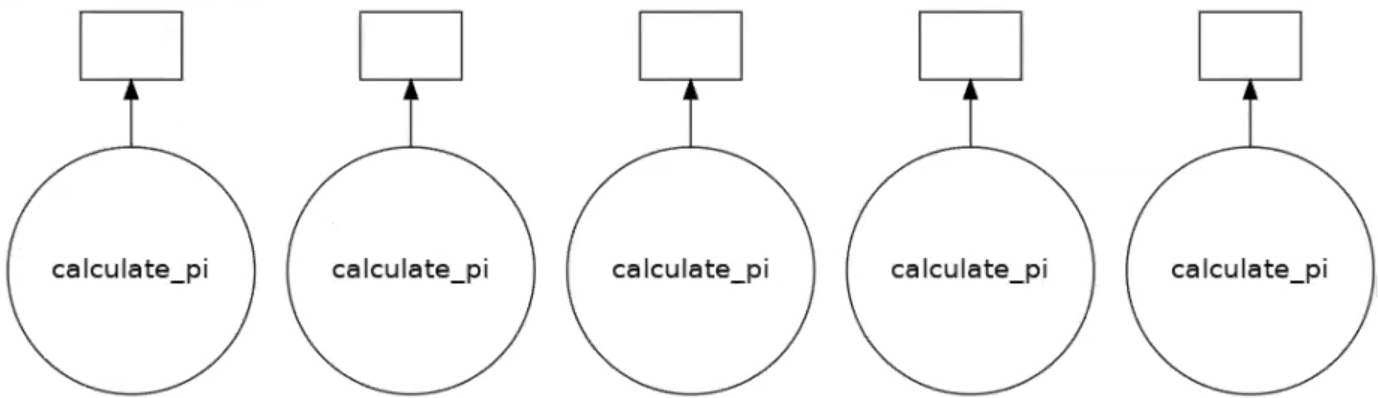
Continuing with Pi calculation
Run the same
calculate_pifunction for array sizes 1GB-5GB. Time the numpy only version against when using dask. Do you notice anything? Modify the codes in the notebook and submit to the queue.You should have 5 different runs, 1GiB, 2GiB, 3GiB, 4GiB and 5GiB.
Solution
import dask
from dask.distributed import Client
import numpy as np
import time

def calculate_pi(size_in_bytes):

    """Calculate pi using a Monte Carlo method."""

    rand_array_shape = (int(size_in_bytes / 8 / 2), 2)

    # 2D random array with positions (x, y)
    xy = np.random.uniform(low=0.0, high=1.0, size=rand_array_shape)

    # check if position (x, y) is in unit circle
    xy_inside_circle = (xy ** 2).sum(axis=1) < 1

    # pi is the fraction of points in circle x 4
    pi = 4 * xy_inside_circle.sum() / xy_inside_circle.size

    print(f"\nfrom {xy.nbytes / 1e9} GB randomly chosen positions")
    print(f"   pi estimate: {pi}")
    print(f"   pi error: {abs(pi - np.pi)}\n")

    return pi

if __name__ == '__main__':

# Numpy only version
    t0 = time.time()
    for i in range(5):
       pi1 = calculate_pi(1000000000*(i+1))
    t1 = time.time()
    print(f"time taken for nupmy is {t1-t0}\n\n")

# Dask version
    client = Client(n_workers=5, threads_per_worker=1, memory_limit='50GB')
    client

    t0 = time.time()
    results = []
    for i in range(5):
       dask_calpi = dask.delayed(calculate_pi)(1000000000*(i+1))
       results.append(dask_calpi)
    dask.compute(*results)
    t1 = time.time()
    print("time taken for dask w5/t1 is " + str(t1-t0))

    client.close()
Dask Array
From the previous example parallelisation comes with a downside. If we have 1 task that needs 10GB memory, having 10 simultaneously will need 100GB in total. Each Kay node has 180GB of memory, what if we need more than that? Dask Array splits a larger array into smaller chunks. We can work on larger than memory arrays but still use all of the cores. You can think of the Dask array as a set of smaller numpy arrays.

Below we have some simple examples of using dask arrays. Again we need to setup a LocalCluster.
client = Client(n_workers=2, threads_per_worker=1, memory_limit='1GB')
client

import dask.array as da
These examples courtesy of Dask contributor James Bourbeau
a_np = np.arange(1, 50, 3)   # Create array with numbers 1->50 but with a stride of 3
print(a_np)
a_np.shape
[ 1 4 7 10 13 16 19 22 25 28 31 34 37 40 43 46 49]
(17,)
That’s the NumPy version. For dask we will set up an array of the same size, but in chunks of size = 5.
a_da = da.arange(1, 50, 3, chunks=5)
a_da
As an output we get a diagram.
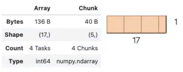
Notice that we split the 1D array into 4 chunks with a maximum size of 5 elements. Also that Dask is smart enough to have setup a set of tasks.
print(a_da.dtype)
print(a_da.shape)
print(a_da.chunks)
print(a_da.chunksize)
int64
(17,)
((5, 5, 5, 2),)
(5,)
As before we can visualise this task graph
a_da.visualize()
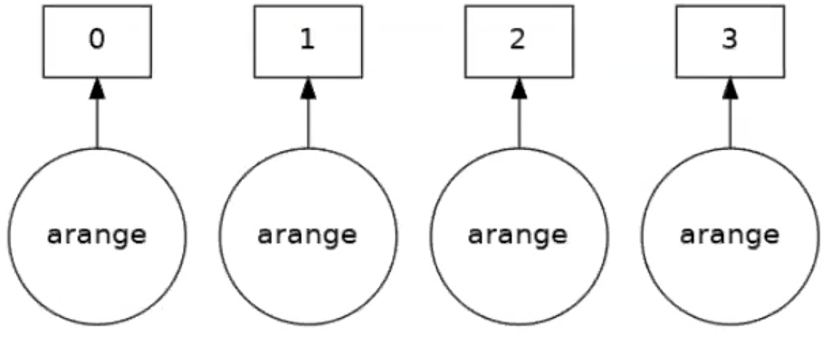
Four tasks have been created for each of the subarrays. Take an operation where the tasks are independent. When the array is created it will be executed in parallel. Now say we want to square the elements of the array, and look at the task graph of that
(a_da ** 2).visualize()
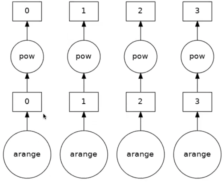
Up to now we have only been setting up the task graph or how the workload is split. Remember, we haven’t actually done anything yet. To actually perform the set of tasks we need to compute the result.
(a_da ** 2).compute()
array([   1,   16,  100,  169,  256,  361,  484,  625,  784,  961,
       1156, 1369, 1600, 1849, 2116, 2401])
You can see that the parallelisation is easy, you don’t really need to understand the parallelisation strategy or anything at all! A numpy array is returned. There are other operations that can be done.
Dask arrays support a large portion of the NumPy interface such as:
- Arithmetic and scalar mathematics:
+,*,exp,log, … - Reductions along axes:
sum(),mean(),std(),sum(axis=0), … - Tensor contractions / dot products / matrix multiply:
tensordot - Axis reordering / transpose:
transpose - Slicing:
x[:100, 500:100:-2] - Fancy indexing along single axes with lists or numpy arrays:
x[:, [10, 1, 5]] - Array protocols like
__array__and__array_ufunc__ - Some linear algebra:
svd,qr,solve,solve_triangular,lstsq, …
See the Dask array API docs for full details about what portion of the NumPy API is implemented for Dask arrays. You may not be able to do everything on your machine, so check to see what you and your machine are capable of.
Blocked Algorithms
Dask arrays are implemented using blocked algorithms. These algorithms break up a computation on a large array into many computations on smaller pieces of the array. This minimizes the memory load (amount of RAM) of computations and allows for working with larger-than-memory datasets in parallel. Dask supports a large protion of the numpy functions.
The below will generate a random array, and it will automatically create the tasks, and from there the sums will be parallelised. This is similar to what you would see in MPI, but obviosuly much easier to implement
x = da.random.random(20, chunks=5)
# Sets up the computation
result = x.sum()
# result.visualize()
result.compute()
9.83769173433889
When you run the above (uncomment to visualise it), it will be more complex than before, but it is creating the numpy array and doing the partial sums, followed by an aggregate and therefore giving you the answer. We haven’t really done much at all, but have still created a fairly complex set up.
A more complex example
Change the size to a 15x15 array and create a chunks array of size
10, 5. Repeat the above steps, but do it with as the transpose of a matrix,x + x.T.Solution
x = da.random.random(size=(15, 15), chunks=(10, 5)) x.chunks result = (x + x.T).sum() result.visualize() result.compute()222.71576130946The task graph will look a mess, but who cares! It’s done it for us! Don’t forget to close your client!
We can perform computations on larger-than-memory arrays!
client.restart()
client.close()
Calculate pi
Going back to the previous example, calculating pi, how can we go about parallelising the function itself. Well, we could use dask arrays rather than numpy.
So let’s change our 2D random array, xy, and specify the number of chunks in our function.
def dask_calculate_pi(size_in_bytes,nchunks):

    """Calculate pi using a Monte Carlo method."""

    rand_array_shape = (int(size_in_bytes / 8 / 2), 2)
    chunk_size = int(rand_array_shape[0]/nchunks)

    # 2D random array with positions (x, y)
    xy = da.random.uniform(low=0.0, high=1.0, size=rand_array_shape, chunks=chunk_size)
    print(xy)

    # check if position (x, y) is in unit circle
    xy_inside_circle = (xy ** 2).sum(axis=1) < 1

    # pi is the fraction of points in circle x 4
    pi = 4 * xy_inside_circle.sum() / xy_inside_circle.size

    # Do the computation
    result = pi.compute()

    print(f"\nfrom {xy.nbytes / 1e9} GB randomly chosen positions")
    print(f"   pi estimate: {result}")
    print(f"   pi error: {abs(result - np.pi)}\n")

    return result
client = Client(n_workers=5,threads_per_worker=1,memory_limit='1GB')
client
%time dask_calculate_pi(10000000,20)
dask.array<uniform, shape=(625000, 2), dtpye=float64, chunksize=(31250, 2), chunktype=numpy.ndarray>

from 0.01 GB randomly chosen positions
   pi estimate: 3.146176
   pi error: 0.004583346410206968

CPU times: user 486 ms, sys: 176 ms, total: 662 ms
Wall time: 2.34 s

3.146176
Calculating Pi Part 2
Using dask arrays expand the pi calculation to use a 100GB array. This is still smaller than the total memory per node (~180GB). We should be careful in deciding the memory per worker and threads per worker. Modify the code found in the notebook and submit on the compute nodes.
You will need to start the client and run the function.
Solution
import numpy as np
import dask
import dask.array as da
from dask.distributed import Client
import time

def dask_calculate_pi(size_in_bytes,nchunks):

    """Calculate pi using a Monte Carlo method."""

    rand_array_shape = (int(size_in_bytes / 8 / 2), 2)
    chunk_size = int(rand_array_shape[0]/nchunks)
    print(chunk_size)

    # 2D random array with positions (x, y)
    xy = da.random.uniform(low=0.0, high=1.0, size=rand_array_shape, chunks=chunk_size)
    print(f" Created xy\n {xy}\n")
    print(f" Number of partitions/chunks is {xy.numblocks}\n")

    # check if position (x, y) is in unit circle
    xy_inside_circle = (xy ** 2).sum(axis=1) < 1

    # pi is the fraction of points in circle x 4
    pi = 4 * xy_inside_circle.sum() / xy_inside_circle.size

    result = pi.compute()

    print(f"\nfrom {xy.nbytes / 1e9} GB randomly chosen positions")
    print(f"   pi estimate: {result}")
    print(f"   pi error: {abs(result - np.pi)}\n")

    return result

if __name__ == '__main__':

    client = Client(n_workers=5, threads_per_worker=4, memory_limit='40GB')
    print(client)

    t0 = time.time()
    dask_calculate_pi(100000000000,40)
    t1 = time.time()
    print("time taken for dask is " + str(t1-t0))

    client.close()
Feel free to investigate some of the links below.
Dask MPI
Up to now with Dask we have been using a single node. The local cluster is like multi-threading, which, by its nature
will not work on across multiple nodes. The issue is how the workers comminucate with the scheduler. As we have seen we
can use multiple nodes using MPI. Dask MPI is built on top of mpi4py.
When we operate Dask MPI there is another part of the framework that instead of threads, splits the scheduler and workers over MPI processes. The processes are laid out as follows:
- Rank 0 runs the scheduler.
- Rank 1 runs the python script.
- Ranks 2 and above are the workers.
To illustrate how this is done we will use the previous example. Below is the complete python code, and we only need
to import one more package, dask_mpi. The function itself is unchanged from last time when we used dask arrays.
import numpy as np

import dask
import dask.array as da
from dask.distributed import Client
from dask_mpi import initialize
import time

def dask_calculate_pi(size_in_bytes,nchunks):

    """Calculate pi using a Monte Carlo method."""

    rand_array_shape = (int(size_in_bytes / 8 / 2), 2)
    chunk_size = int(rand_array_shape[0]/nchunks)
    print(chunk_size)

    # 2D random array with positions (x, y)
    xy = da.random.uniform(low=0.0, high=1.0, size=rand_array_shape, chunks=chunk_size)
    print(f" Created xy\n {xy}\n")
    print(f" Number of partitions/chunks is {xy.numblocks}\n")


    # check if position (x, y) is in unit circle
    xy_inside_circle = (xy ** 2).sum(axis=1) < 1

    # pi is the fraction of points in circle x 4
    pi = 4 * xy_inside_circle.sum() / xy_inside_circle.size

    result = pi.compute()

    print(f"\nfrom {xy.nbytes / 1e9} GB randomly chosen positions")
    print(f"   pi estimate: {result}")
    print(f"   pi error: {abs(result - np.pi)}\n")

    return result

if __name__ == '__main__':
    initialize(nthreads=4,memory_limit='40GB')

    client = Client()


    t0 = time.time()
    print(client)
    dask_calculate_pi(100000000000,40)
    t1 = time.time()
    print("time taken for dask is " + str(t1-t0))

    close.client()
The changes come in the main body of the code, when we come to initialise it. You will still need to initialise the
scheduler and workers by calling Client. However this time it is called without any arguments. The system of MPI
processes is created by calling intialize. You can see that the parameters are setup at this call and not through
Client(). One thing you may notice is that the number of workers has not been set. This is set at execute time.
Below is an example slurm script, from which we can set the number of workers.
#!/bin/bash
#SBATCH --nodes=2
#SBATCH --time=01:00:00
#SBATCH -A $ACCOUNT
#SBATCH --job-name=calpi
#SBATCH -p $PARTITION
#SBATCH --reservation=$RESERVATION


module purge
module load conda openmpi/gcc/3.1.2
module list

source activate /ichec/home/users/course00/conda_HPC

cd $SLURM_SUBMIT_DIR


mpirun -n 6 -npernode 3 python -u dask_MPI_calculate_pi.py

exit 0
The number of workers has been set by the number of processes we create. In this case it is 4 because rank 0 is the scheduler and rank 1 runs the python script. The workers come into play when there are parallel tasks to run. Just to prove that it will work over multiple nodes we have asked for 3 processes to run per node. This version is not faster than using plain Dask but it allows more memory per worker.
The output will come in a slurm output, and there will be a lot of material in the output file in addition to the result.
Prove it!
Run the above to make sure that it all works. Remember that you cannot run this example through the notebook. Be sure to run the slurm script and specify the account, partition and reservation outlined to you by your instructor.
Key Points
Dask allows task parallelisation of problems
Identification of tasks is crucial and understanding memory usage
Dask Array is a method to create a set of tasks automatically through operations on arrays
Tasks are created by splitting larger arrays, meaning larger memory problems can be handled
GPUs with Python
Overview
Teaching: 30 min
Exercises: 25 minQuestions
What is a GPU?
What is CUDA?
How can I submit a job to a GPU?
Objectives
Gain understanding of how a GPU works
Implement Dask GPU
![]()
Basics of GPUs
If you’re taking this course, it is quite probable that you have never come across GPUs before. This section will help give an overview into one of the most important bits of hardware in computing. A GPGPU is a device that is external to the machine CPU but can perform computation. The benefits of using a GPU is that it has many more cores (thousands!) than a CPU which are more efficient at particular operations. ICHEC’s cluster, Kay, has Tesla VT100 which have 5120 CUDA cores. This is a stark comparison to a node on Kay, which only has 40 CPU cores.
These cores are arranged in streaming multiprocessors (SM) of which there are 80. The downsides are that GPU cores are not as flexible as CPU cores. Data needs to be moved between CPU and GPU memory, increasing overheads. The memory per GPU core is tiny compared to that of the CPU. The total memory of a Tesla VT100 is only 16 GiB. So you need to be very conscious of how you use the memory in any code that you write on a GPU.
GPGPUs are best when performing SIMD (single input, multiple data) calculations, due to the fact that groups of cores can only perform a single instruction at any one time.

CUDA Basics
CUDA is not a language in itself but are extensions to C. Similar to MPI where an individual process runs on an individual core, the same applies here, as does the fact that the code runs the same on each process. There is a single source code which defines which computation is done on the CPU and which on the GPU. The CPU controls the flow of the execution. The CPU is called the host and the GPU the device.
The host runs C functions defined the same way as normal. The device runs what are called kernels which are similar to C functions. The execution model is thread based similar to OpenMP. Each kernel has a grid and grids are organised into blocks. Each block has a number of threads. One block is executed on a single SM, so there is a maximum number of threads a block can have. These constructions can be 1D,2D, or 3D. The example below is a 2D grid.
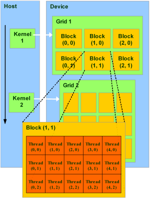
How to explore your GPU
For each GPU node on Kay there are 2 Tesla VT100s which have 16GB memory each. One way to access the GPUs from Python is by using the package
pycuda. Through this we can examine them. The login nodes do not have GPUs, so we need to submit the script below to theGpuQ.Take a note of the command used and submit it to the
GpuQ. What does the output look like? What are the most important lines in the output?import pycuda.driver as drv drv.init() drv.get_version() devn = drv.Device.count() print ('Localized GPUs =',devn) sp = drv.Device(0) print ('Name = ',sp.name()) print ('PCI Bus = ',sp.pci_bus_id()) print ('Compute Capability = ',sp.compute_capability()) print ('Total Memory = ',sp.total_memory()/(2.**20) , 'MBytes') attr = sp.get_attributes() for j in range(len(attr.items())): print (list(attr.items())[j])#,'Bytes (when apply)' print ('------------------') print ('------------------')#!/bin/bash #SBATCH --nodes=1 #SBATCH --time=00:10:00 #SBATCH -A $ACCOUNT #SBATCH --job-name=test #SBATCH -p GpuQ #SBATCH --reservation=$RESERVATION module purge module load conda cuda/11.4 gcc/8.2.0 module list source activate /ichec/home/users/course00/conda_HPC cd $SLURM_SUBMIT_DIR python -u gpu_test.py exit 0Output
Below is the output from this script. We have highlighted a few of the key items have been extracted. You can see the maximum block and grid sizes. Notice that there is a maximum number of threads per block. At the bottom you can see the wrap size. Threads in a wrap are constrained to run the same instruction/operation at any one time. Block sizes should be a multiple of the wrap size.
Name =  Tesla V100-PCIE-16GB
PCI Bus =  0000:5E:00.0
Compute Capability =  (7, 0)
Total Memory =  16130.5 MBytes
(pycuda._driver.device_attribute.ASYNC_ENGINE_COUNT, 7)
...
(pycuda._driver.device_attribute.MAX_BLOCK_DIM_X, 1024)
(pycuda._driver.device_attribute.MAX_BLOCK_DIM_Y, 1024)
(pycuda._driver.device_attribute.MAX_BLOCK_DIM_Z, 64)
(pycuda._driver.device_attribute.MAX_GRID_DIM_X, 2147483647)
(pycuda._driver.device_attribute.MAX_GRID_DIM_Y, 65535)
(pycuda._driver.device_attribute.MAX_GRID_DIM_Z, 65535)
...
(pycuda._driver.device_attribute.MAX_THREADS_PER_BLOCK, 1024)
...
(pycuda._driver.device_attribute.WARP_SIZE, 32)
The main things to point out are the
MAX_BLOCK_DIM, andMAX_GRID_DIM, which are the maximum size of the blocks and the grid sizes that you can have in all dimensions. Additionally is theMAX_THREADS_PER_BLOCK, which will limit the size of the block. TheWARP_SIZEis important as it means that the number of CUDA cores are split into 32 core blocks and each thread within the block/unit need to work on a single instruction. 32 cores are “tied togethter” throughout the GPU. When designing your blocks, you want to make sure that they are a multiple of theWARP_SIZE(64, 96, 128, 160, 320, 640, 1024, etc) to ensure the code is efficient.
Vector addition
A typical example of using a GPU to perform work is vector addition. This is a trivially parallelizable example because the operation for each element of the array is independent. We will look at how this is done in C.
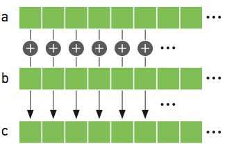
#include <stdio.h>
#include <stdlib.h>

int main(void)
{
    int N = 10;
    float *a,*b,*c;

    // Reserve memory
    a = (float *) malloc(N * sizeof(float));
    b = (float *) malloc(N * sizeof(float));
    c = (float *) malloc(N * sizeof(float));


    // Initialize arrays
    for (int i = 0; i < N; ++i){
        a[i] = i;
        b[i] = 2.0f;
    }


    // Perform vector addition
    for (int i = 0; i < N; ++i){
        c[i]= a[i]+b[i];
    }

    printf("Done %f\n",c[0]);

    // Free arrays
    free(a); free(b); free(c);
    return 0;
}
Don’t worry if your C knowledge isn’t up to scratch, but the main points are as follows:
- We need to reserve the memory for
a,b, andcin the CPU to hold the arrays, of sizeN - Initialise the arrays
- Perform our vector addition
- Free the memory that we have reserved.
An individual thread is identified through the block ID and the thread ID within the block. In the example below,
which is 1-dimensional (1x5), we have 3 blocks and 15 threads each. Within each block our threadIdx are 0-4. To get
the global threadId we need to perform the sum as shown.
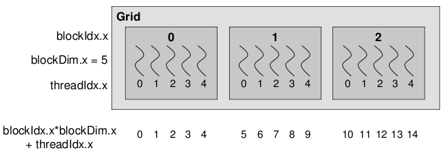
Below is the CUDA version of vector addition. The vectorAdd function is the CUDA kernel. Notice that there is no for
loop. It is written as if for a single thread. A single threads adds a single element, that element is determined by
the thread and block IDs.
To compile this code we use nvcc.
#include <stdio.h>
#include <stdlib.h>
#include <cuda_runtime.h>
// CUDA Kernel
__global__ void vectorAdd(const float *A, const float *B, float *C, int numElements)
{
    int i = blockDim.x * blockIdx.x + threadIdx.x;
    if (i < numElements)
    {
        C[i] = A[i] + B[i];
    }
}

/*
 * Host main routine
 */
int main(void)
{
    int numElements = 15;
    size_t size = numElements * sizeof(float);
    printf("[Vector addition of %d elements]\n", numElements);

    float *a,*b,*c;
    float *a_gpu,*b_gpu,*c_gpu;

    // Reserve host memory
    a = (float *) malloc(size);
    b = (float *) malloc(size);
    c = (float *) malloc(size);

    // Reserve device memory
    cudaMalloc((void **)&a_gpu, size);
    cudaMalloc((void **)&b_gpu, size);
    cudaMalloc((void **)&c_gpu, size);

    // Initialize arrays
    for (int i=0;i<numElements;++i ){
    	a[i] = i;
    	b[i] = 2.0f;
    }

    // Copy the host input vectors A and B in host memory to the device input vectors in
    // device memory
    printf("Copy input data from the host memory to the CUDA device\n");
    cudaMemcpy(a_gpu, a, size, cudaMemcpyHostToDevice);
    cudaMemcpy(b_gpu, b, size, cudaMemcpyHostToDevice);

    // Launch the Vector Add CUDA Kernel
    int threadsPerBlock = 256;
    int blocksPerGrid =(numElements + threadsPerBlock - 1) / threadsPerBlock;
    printf("CUDA kernel launch with %d blocks of %d threads\n", blocksPerGrid, threadsPerBlock);
    vectorAdd<<<blocksPerGrid, threadsPerBlock>>>(a_gpu, b_gpu, c_gpu, numElements);

    // Copy the device result vector in device memory to the host result vector
    // in host memory.
    printf("Copy output data from the CUDA device to the host memory\n");
    cudaMemcpy(c, c_gpu, size, cudaMemcpyDeviceToHost);

    for (int i=0;i<numElements;++i ){
    	printf("%f \n",c[i]);
    }

    // Free host memory
    free(a); free(b); free(c);

    // Free device global memory
    cudaFree(a_gpu);
    cudaFree(b_gpu);
    cudaFree(c_gpu);

    printf("Done\n");
    return 0;
}
In the example above we have an array of length = 15, we reserve the memory on the GCPU then on the GPU as they are two
distinct memories. We copy over the data from the GPU over to the GPU for a and b from host (CPU) to device (GPU).
The device is the one that does the vector addition, and stores the result in c_gpu. We then copy that back from the
device to the host. It’s a bit more complex now with CUDA, then we free the memory on the CPU and GPU.
The functions are also different and defined in the CUDA environment. The other thing to note is that the GPU kernel
itself is defined by __global__ void vectorAdd(...). We give it the a, b and c vectors as well as the number of
elements. There is no loops in the code, and we are writing it as if for a single thread. But the thing we need to make
sure of is which thread is working on which element of the array, and that they only work on a single element of the
array. If we have more threads than number of elements, we also need to check for that as well.
PyCUDA
So far we have been using the GPUs through cuda code. PyCUDA is a framework which allows us to access the GPU form a python environment. There are different ways to achieve this. First we will look at GPUArrays, as we can copy arrays from the host to device, perform basic operations then return the data to the host.
The code below does the same as those above. Much of the work is hidden, like python itself. Also you can view the data both on the CPU and GPU. The distinction between what is on the GPU and CPU is blurred which may cause problems.
from pycuda import autoinit
from pycuda import gpuarray
import numpy as np


# Create single precision host arrays
aux = range(15)
a = np.array(aux).astype(np.float32)
b = 2.0*np.ones(len(aux),dtype=np.float32)

# Create and copy data to GPU
a_gpu = gpuarray.to_gpu(a)
b_gpu = gpuarray.to_gpu(b)

# Perform operation on GPU
aux_gpu = a_gpu+b_gpu

# Return data to host
c = aux_gpu.get()

print("a_gpu=")
print(a_gpu)

print("b_gpu=")
print(b_gpu)

print("aux_gpu=")
print(type(aux_gpu))
print(aux_gpu)

print("c=")
print(type(c))
print(c)

# Free memory on GPU - 2 methods
del(a_gpu)
b_gpu.gpudata.free()
This code cannot be run in notebooks, so the terminal is essential here.
PyCUDA
Run the above code by submitting it to the
GpuQ.
Using source code
The second way to go about doing it is to use the CUDA kernel that we created, rather than turning it into Python. You may have a CUDA code, but would prefer if it stayed in CUDA which you can then use. However notice that we are only using the kernel.
from pycuda import autoinit
from pycuda import gpuarray
import pycuda.driver as drv
import numpy as np
from pycuda.compiler import SourceModule

# Read in source code
cudaCode = open("vecadd.cu","r")
myCUDACode = cudaCode.read()
myCode = SourceModule(myCUDACode)

# Extract vectorAdd kernel
importedKernel = myCode.get_function("vectorAdd")

# Create host arrays
aux = range(15)
a = np.array(aux).astype(np.float32)
b = 2.0*np.ones(len(aux),dtype=np.float32)
c = np.zeros(len(aux),dtype=np.float32)

# Create and copy data to GPU, need to three arrays as there are three arguments to vectorAdd
a_gpu = gpuarray.to_gpu(a)
b_gpu = gpuarray.to_gpu(b)
c_gpu = gpuarray.to_gpu(c)

# Set grid/block properties
threadsPerBlock = 256
blocksPerGrid = (len(aux) + threadsPerBlock - 1) / threadsPerBlock;


# Perform operation
# Need to give the number of blocks per grid in 3D
# Need to give block size in 3D
importedKernel(a_gpu.gpudata,b_gpu.gpudata,c_gpu.gpudata,block=(threadsPerBlock,blocksPerGrid,1),grid=(1,1,1))

# Wait for computation to finish
drv.Context.synchronize()

#
c = c_gpu.get()
print(c=")
print(c)
We can grab the kernel vectorAdd from our CUDA code, and then we do similar to what was done previously, creating our
“post-arrays”, as well as our empty c array. We then copy those over as we need to make space on the GPU as before.
We also need to create the number of threads per block, which is effectively creating our grid. If you recall, in
previous cases we didn’t need to bother with that. We then call our imported kernel, and can run it this way, adding
the arguments for the GPU, block size etc. We then get our result back again. As you can see, there is more coding
to be done than the first approach using GPUArrays only. But might be necessary for more complex kernels.
Using source code
Run the above code by submitting it to the
GpuQ.
Elementwise Kernels
Yet another way is to use a predefined function ElementwiseKernel.
As its name suggests it performs operations that are trivially parallel across the array.
There are other similar pyCUDA functions.
from pycuda import autoinit
from pycuda import gpuarray
import numpy as np
from pycuda.elementwise import ElementwiseKernel

# Create host arrays
aux = range(15)
a = np.array(aux).astype(np.float32)
b = 2.0*np.ones(len(aux),dtype=np.float32)
c = np.zeros(len(aux),dtype=np.float32)

# Create and copy data to GPU, need to three arrays as there are three arguments to vectorAdd
a_gpu = gpuarray.to_gpu(a)
b_gpu = gpuarray.to_gpu(b)
c_gpu = gpuarray.to_gpu(c)

# Create the function that does vector addition in this case
myCudaFunc = ElementwiseKernel(arguments = "float *a, float *b, float *c",
                               operation = "c[i] = a[i]+b[i]",
                               name = "myVecAdd")
# Execute function
myCudaFunc(a_gpu,b_gpu,c_gpu)

# Return data to host
c = c_gpu.get()

print("c =")
print(c)

# Free memory on GPU
a_gpu.gpudata.free()
b_gpu.gpudata.free()
c_gpu.gpudata.free()
These once again will only work for things like vector addition. The method is similar, but we need to define the arguments to the functions and is generated through the ElementwiseKernel function itself. This approach may run into difficulties for more complex kernels.
Using
ElementwiseKernalRun the above code by submitting it to the
GpuQ.
Dask GPU
So that is how to use GPUs the hard way. Thankfully we can use Dask, which makes it much easier to use. However, it is in its early stages of development. It is very easy to setup.
Let us use the example we had previously calculating pi. The only difference is that we setup a LocalCUDACluster. This then uses both GPUs as the workers.
Our example we have here is much slower than the CPU version. Some example will work better than others, but it is clear that specific problems will be accelerated using this approach.
But using Dask array we have been able to work on an array much larger than the GPU memory, so although this example can technically work, having an understanding of memory usage will be important when dealing with problems like this.
import numpy as np

import dask
import dask.array as da
from dask.distributed import Client
from dask_cuda import LocalCUDACluster         # Added

import time


def dask_calculate_pi(size_in_bytes,nchunks):

    """Calculate pi using a Monte Carlo method."""

    rand_array_shape = (int(size_in_bytes / 8 / 2), 2)
    chunk_size = int(rand_array_shape[0]/nchunks)
    print(chunk_size)

    # 2D random array with positions (x, y)
    xy = da.random.uniform(low=0.0, high=1.0, size=rand_array_shape, chunks=chunk_size)
    print(f" Created xy\n {xy}\n")
    print(f" Number of partitions/chunks is {xy.numblocks}\n")


    # check if position (x, y) is in unit circle
    xy_inside_circle = (xy ** 2).sum(axis=1) < 1

    # pi is the fraction of points in circle x 4
    pi = 4 * xy_inside_circle.sum() / xy_inside_circle.size

    result = pi.compute()

    print(f"\nfrom {xy.nbytes / 1e9} GB randomly chosen positions")
    print(f"   pi estimate: {result}")
    print(f"   pi error: {abs(result - np.pi)}\n")

    return result


if __name__ == '__main__':

    cluster = LocalCUDACluster()             # Added
    print(cluster)

    client = Client(cluster)
    print(client)

    t0 = time.time()
    dask_calculate_pi(100000000000,40)
    t1 = time.time()
    print("time taken for dask is " + str(t1-t0))

    client.restart()
    client.close()
We need to add a line that sets up the cluster as a LocalCUDACluster(), the client, then we run our code and get
the result at the end.
Using
ElementwiseKernalRun the above code by submitting it to the
GpuQ.
Although it is clear that we can access GPUs from Python, there is a tradeoff between ease of use and flexibility. GPUs are more difficult to generate speedups over multithreading, but thankfully there are packages and frameworks that have already been optimised for GPUs, a key example being TensorFlow.
Additional links
Feel free to check out some of the material below.
Key Points
GPUs are more powerful than CPUs, and have several thousand cores, but have much less memory