Dask
Overview
Teaching: 60 min
Exercises: 30 minQuestions
What is Dask?
How can I implement Dask array?
How can I use Dask MPI
Objectives
Implement Dask array
Implement Dask MPI
![]()
Dask
Dask is a framework that covers many things which were not possible even a few years ago. It allows us to create
multiple tasks with a minimum of effort. There are different aspects to Dask of which we will cover just a few during
this lesson. Dask is integrated with different projects such as pandas, numpy and scipy. This allows
parallelisation of for example scipy functions with minimum changes to the python code. Some of the projects have
their own multithreaded functions, so Dask is not essential.
Dask can work very well in notebook environments, as it gives you a good visual representation as to what is going on. You can open up the notebook for this episode.
We will first look at “Dask Distributed”. The first step is to create a set of workers with a scheduler. Here we are creating 2 “worker” processes with 2 threads each. This means that we can assign a particular task to a specific worker. There will be 1GB for all workers.
import dask
from dask.distributed import Client

client = Client(n_workers=2, threads_per_worker=2, memory_limit='1GB')

client
The Client function is needed here to set up a variable which we will call lowercase client. It is worth noting
that this is running on a login node, hence the memory size is small as we do not want to stress the system. As you can
see upon running the cell with (using the correct environment) your output will be very different to what you may
expect.
It will display some information about:
Client:
- Connection Method
- Cluster type
- Dashboard
And in the dropdown menu on Cluster Info: Local Cluster
- Dashboard
http://127.0.0.1:12345/status - Total threads: 4
- Status: running
- Workers: 2
- Total memory: 1.86 GiB
- Using processes: True
And in the second drop down menu about the scheduler Scheduler
- Comm:
... - Dashboard:
http://127.0.0.1:12345/status - Started: just now
- Workers: 2
- Total threads: 4
- Total memory: 1.86 GiB
Further information is then displayed about the two workers. This information is not essential, but can help you understand what is being set up.
Clicking the link in Dashboard will not work on its own. To deal with this you would need to set up an ssh tunnel through the machine that you are using the terminal.
$ ssh -N -L 8787:localhost:12345 youraccount@login1@kay.ichec.ie
You may be using Jupyter notebook already, which will be taking up the port 8080, so we can change that in the
terminal to 8787 as shown above. The second thing to change is the port that is being used on your host/machine. If
you look up at the Dashboard link, the final 5 numbers will show the port, in this case 12345. Yours may show up
differently.
Upon entering the required passwords, your tunnel is set up and you can view your Dashboard. Entering localhost:8787
into your web browser will produce something similar to below.
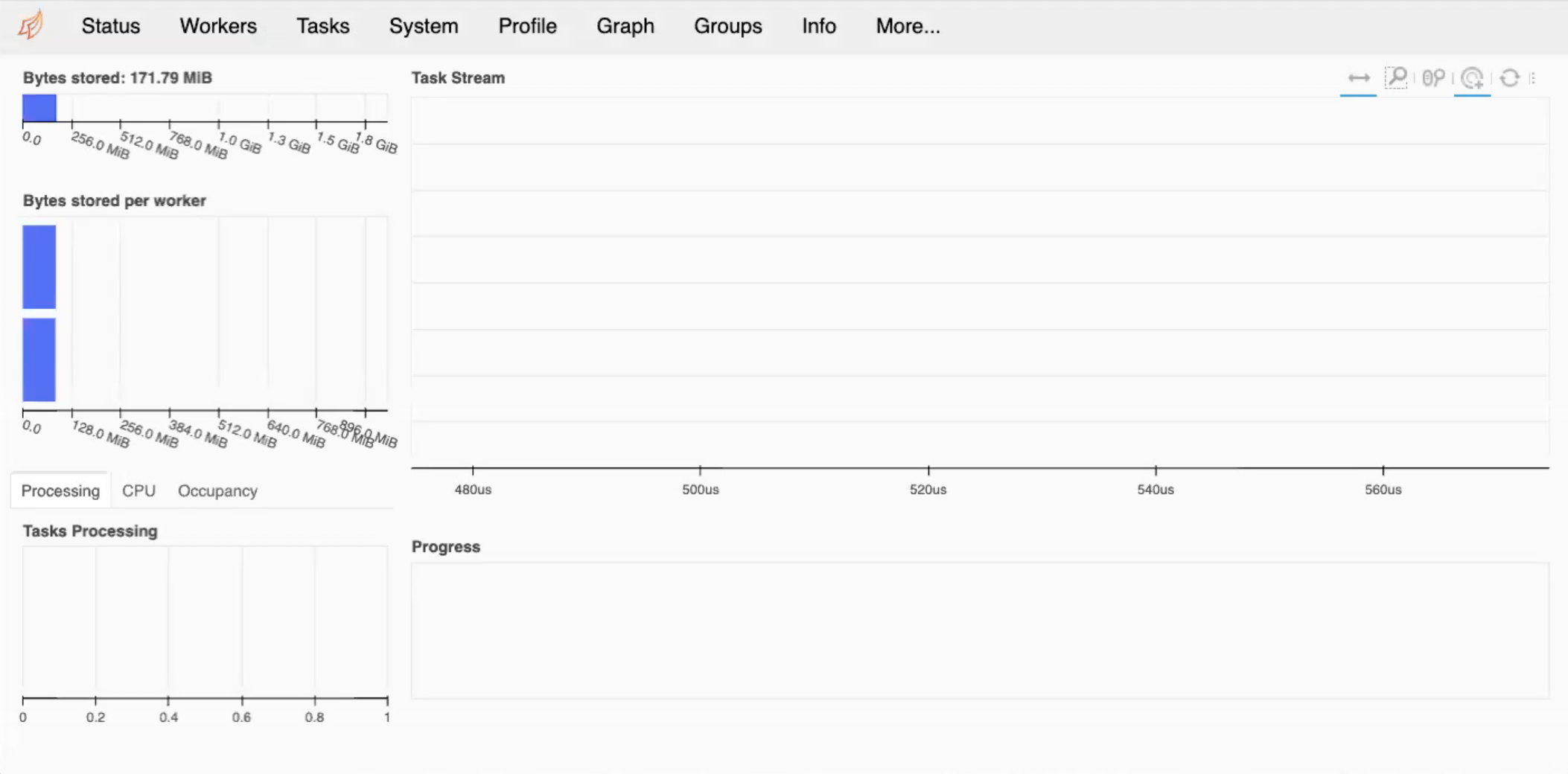
If you are doing debugging of your system and seeing what is going on with load balancing, then this can be very useful, giving you the amount of memory per worker and so on. If your program exceeds the memory usage specified in the code, then naturally, you will get some errors.
Dask Dashboard
Ensure that you have followed the above steps and take some time to explore around the Dashboard. What do you think everything means, and how can you best utilise them?
The alternative to the above method is to install jupyter-server-proxy.
Once we are finished with this we need to close the client, and therefore you will stop the workers.
client.close()
Using this type of cluster will however restrict you to a single node of your machine. We can use more than one node later on.
Here we have a simple example where we estimate pi. This version uses numpy functions to perform the calculations. Note there are no explicit loops. The code is serial. We are instead setting up an array, setting it up where we are asked for the size of array that we want to use. As the array gets bigger, our estiamte of pi will improve. As we are using NumPy to make it more efficient, we don’t necessarily need any loops.
import numpy as np

def calculate_pi(size_in_bytes):

    """Calculate pi using a Monte Carlo method."""

    rand_array_shape = (int(size_in_bytes / 8 / 2), 2)

    # 2D random array with positions (x, y)
    xy = np.random.uniform(low=0.0, high=1.0, size=rand_array_shape)

    # check if position (x, y) is in unit circle
    xy_inside_circle = (xy ** 2).sum(axis=1) < 1

    # pi is the fraction of points in circle x 4
    pi = 4 * xy_inside_circle.sum() / xy_inside_circle.size

    print(f"\nfrom {xy.nbytes / 1e9} GB randomly chosen positions")
    print(f"   pi estimate: {pi}")
    print(f"   pi error: {abs(pi - np.pi)}\n")

    return pi
%time calculate_pi(10000)
from 1e-05 GB randomly chosen positions
   pi estimate: 3.072
   pi error: 0.06959265358979305

CPU times: user 2.06 ms, sys: 1.44 ms, total: 3.5ms
Wall time: 2.78 ms

3.072
Without needing to change the function we can use Dask to parallelise the work. In this case we have two workers. The
dask.delayed creates a task graph, which creates the tasks that have to be run, if there are more than 2, they need
to be set to run using the scheduler until all tasks are complete. This doesn’t run the task itself however.
The running of the tasks itself is done using dask.compute
client = Client(n_workers=2, threads_per_worker=2, memory_limit='1GB')
dask_calpi = dask.delayed(calculate_pi)(10000)
Runtime with Dask
Check the output of the line below.
%time dask.compute(dask_calpi)Is this what you would expect? Why?
Result
CPU times: user 195 ms, sys: 343 ms, total: 538 ms
Wall time: 546 ms
(3.1488,)
You should find that it is taking longer with Dask! You can change the size of the problem but still find that Dask is slower. This is because we are using Dask incorrectly, the function cannot be divided into tasks. There are also a lot of overheads, which can still slow things down more.
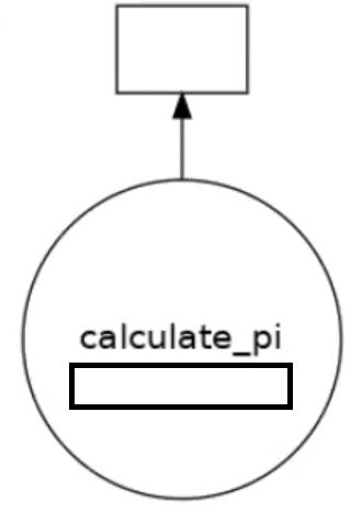
We can visualise how the tasks are decomposed with the visualize function.
dask.visualize(dask_calpi)
You will get an output similar to below, which shows we are only using 1 task. We need to split our workload into multiple tasks.
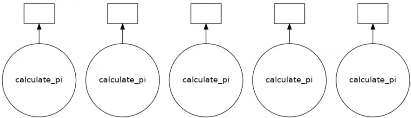
We can only get task parallelism if we call the function more than once. Below is an example of this.
results = []
for i in range(5):
    dask_calpi = dask.delayed(calculate_pi)(10000*(i+1))
    results.append(dask_calpi)

dask.visualize(results)

#to run all the tasks use
#dask.compute(*results)
Running this will produce the following output, now with 5 tasks.
Continuing with Pi calculation
Run the same
calculate_pifunction for array sizes 1GB-5GB. Time the numpy only version against when using dask. Do you notice anything? Modify the codes in the notebook and submit to the queue.You should have 5 different runs, 1GiB, 2GiB, 3GiB, 4GiB and 5GiB.
Solution
import dask
from dask.distributed import Client
import numpy as np
import time

def calculate_pi(size_in_bytes):

    """Calculate pi using a Monte Carlo method."""

    rand_array_shape = (int(size_in_bytes / 8 / 2), 2)

    # 2D random array with positions (x, y)
    xy = np.random.uniform(low=0.0, high=1.0, size=rand_array_shape)

    # check if position (x, y) is in unit circle
    xy_inside_circle = (xy ** 2).sum(axis=1) < 1

    # pi is the fraction of points in circle x 4
    pi = 4 * xy_inside_circle.sum() / xy_inside_circle.size

    print(f"\nfrom {xy.nbytes / 1e9} GB randomly chosen positions")
    print(f"   pi estimate: {pi}")
    print(f"   pi error: {abs(pi - np.pi)}\n")

    return pi

if __name__ == '__main__':

# Numpy only version
    t0 = time.time()
    for i in range(5):
       pi1 = calculate_pi(1000000000*(i+1))
    t1 = time.time()
    print(f"time taken for nupmy is {t1-t0}\n\n")

# Dask version
    client = Client(n_workers=5, threads_per_worker=1, memory_limit='50GB')
    client

    t0 = time.time()
    results = []
    for i in range(5):
       dask_calpi = dask.delayed(calculate_pi)(1000000000*(i+1))
       results.append(dask_calpi)
    dask.compute(*results)
    t1 = time.time()
    print("time taken for dask w5/t1 is " + str(t1-t0))

    client.close()
Dask Array
From the previous example parallelisation comes with a downside. If we have 1 task that needs 10GB memory, having 10 simultaneously will need 100GB in total. Each Kay node has 180GB of memory, what if we need more than that? Dask Array splits a larger array into smaller chunks. We can work on larger than memory arrays but still use all of the cores. You can think of the Dask array as a set of smaller numpy arrays.

Below we have some simple examples of using dask arrays. Again we need to setup a LocalCluster.
client = Client(n_workers=2, threads_per_worker=1, memory_limit='1GB')
client

import dask.array as da
These examples courtesy of Dask contributor James Bourbeau
a_np = np.arange(1, 50, 3)   # Create array with numbers 1->50 but with a stride of 3
print(a_np)
a_np.shape
[ 1 4 7 10 13 16 19 22 25 28 31 34 37 40 43 46 49]
(17,)
That’s the NumPy version. For dask we will set up an array of the same size, but in chunks of size = 5.
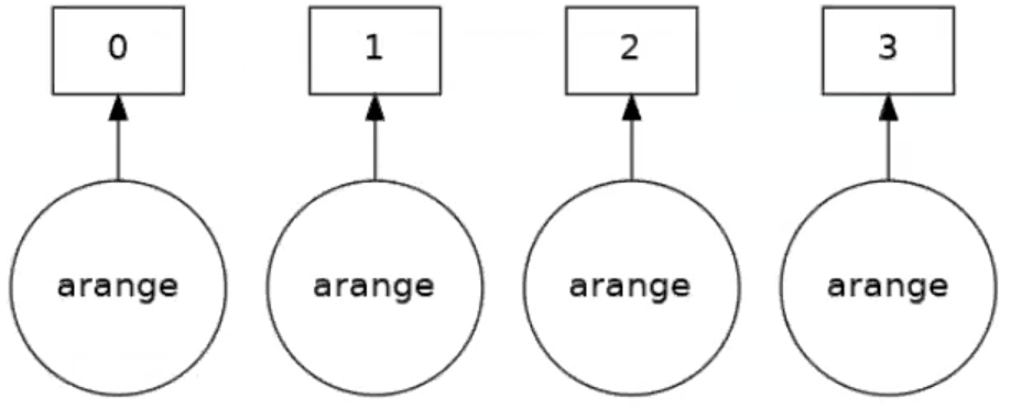
a_da = da.arange(1, 50, 3, chunks=5)
a_da
As an output we get a diagram.
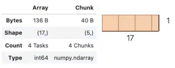
Notice that we split the 1D array into 4 chunks with a maximum size of 5 elements. Also that Dask is smart enough to have setup a set of tasks.
print(a_da.dtype)
print(a_da.shape)
print(a_da.chunks)
print(a_da.chunksize)
int64
(17,)
((5, 5, 5, 2),)
(5,)
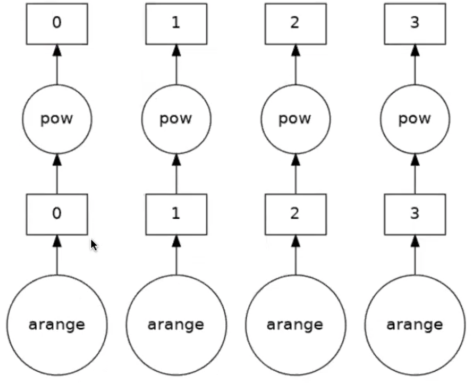
As before we can visualise this task graph
a_da.visualize()
Four tasks have been created for each of the subarrays. Take an operation where the tasks are independent. When the array is created it will be executed in parallel. Now say we want to square the elements of the array, and look at the task graph of that
(a_da ** 2).visualize()
Up to now we have only been setting up the task graph or how the workload is split. Remember, we haven’t actually done anything yet. To actually perform the set of tasks we need to compute the result.
(a_da ** 2).compute()
array([   1,   16,  100,  169,  256,  361,  484,  625,  784,  961,
       1156, 1369, 1600, 1849, 2116, 2401])
You can see that the parallelisation is easy, you don’t really need to understand the parallelisation strategy or anything at all! A numpy array is returned. There are other operations that can be done.
Dask arrays support a large portion of the NumPy interface such as:
- Arithmetic and scalar mathematics:
+,*,exp,log, … - Reductions along axes:
sum(),mean(),std(),sum(axis=0), … - Tensor contractions / dot products / matrix multiply:
tensordot - Axis reordering / transpose:
transpose - Slicing:
x[:100, 500:100:-2] - Fancy indexing along single axes with lists or numpy arrays:
x[:, [10, 1, 5]] - Array protocols like
__array__and__array_ufunc__ - Some linear algebra:
svd,qr,solve,solve_triangular,lstsq, …
See the Dask array API docs for full details about what portion of the NumPy API is implemented for Dask arrays. You may not be able to do everything on your machine, so check to see what you and your machine are capable of.
Blocked Algorithms
Dask arrays are implemented using blocked algorithms. These algorithms break up a computation on a large array into many computations on smaller pieces of the array. This minimizes the memory load (amount of RAM) of computations and allows for working with larger-than-memory datasets in parallel. Dask supports a large protion of the numpy functions.
The below will generate a random array, and it will automatically create the tasks, and from there the sums will be parallelised. This is similar to what you would see in MPI, but obviosuly much easier to implement
x = da.random.random(20, chunks=5)
# Sets up the computation
result = x.sum()
# result.visualize()
result.compute()
9.83769173433889
When you run the above (uncomment to visualise it), it will be more complex than before, but it is creating the numpy array and doing the partial sums, followed by an aggregate and therefore giving you the answer. We haven’t really done much at all, but have still created a fairly complex set up.
A more complex example
Change the size to a 15x15 array and create a chunks array of size
10, 5. Repeat the above steps, but do it with as the transpose of a matrix,x + x.T.Solution
x = da.random.random(size=(15, 15), chunks=(10, 5)) x.chunks result = (x + x.T).sum() result.visualize() result.compute()222.71576130946The task graph will look a mess, but who cares! It’s done it for us! Don’t forget to close your client!
We can perform computations on larger-than-memory arrays!
client.restart()
client.close()
Calculate pi
Going back to the previous example, calculating pi, how can we go about parallelising the function itself. Well, we could use dask arrays rather than numpy.
So let’s change our 2D random array, xy, and specify the number of chunks in our function.
def dask_calculate_pi(size_in_bytes,nchunks):

    """Calculate pi using a Monte Carlo method."""

    rand_array_shape = (int(size_in_bytes / 8 / 2), 2)
    chunk_size = int(rand_array_shape[0]/nchunks)

    # 2D random array with positions (x, y)
    xy = da.random.uniform(low=0.0, high=1.0, size=rand_array_shape, chunks=chunk_size)
    print(xy)

    # check if position (x, y) is in unit circle
    xy_inside_circle = (xy ** 2).sum(axis=1) < 1

    # pi is the fraction of points in circle x 4
    pi = 4 * xy_inside_circle.sum() / xy_inside_circle.size

    # Do the computation
    result = pi.compute()

    print(f"\nfrom {xy.nbytes / 1e9} GB randomly chosen positions")
    print(f"   pi estimate: {result}")
    print(f"   pi error: {abs(result - np.pi)}\n")

    return result
client = Client(n_workers=5,threads_per_worker=1,memory_limit='1GB')
client
%time dask_calculate_pi(10000000,20)
dask.array<uniform, shape=(625000, 2), dtpye=float64, chunksize=(31250, 2), chunktype=numpy.ndarray>

from 0.01 GB randomly chosen positions
   pi estimate: 3.146176
   pi error: 0.004583346410206968

CPU times: user 486 ms, sys: 176 ms, total: 662 ms
Wall time: 2.34 s

3.146176
Calculating Pi Part 2
Using dask arrays expand the pi calculation to use a 100GB array. This is still smaller than the total memory per node (~180GB). We should be careful in deciding the memory per worker and threads per worker. Modify the code found in the notebook and submit on the compute nodes.
You will need to start the client and run the function.
Solution
import numpy as np
import dask
import dask.array as da
from dask.distributed import Client
import time

def dask_calculate_pi(size_in_bytes,nchunks):

    """Calculate pi using a Monte Carlo method."""

    rand_array_shape = (int(size_in_bytes / 8 / 2), 2)
    chunk_size = int(rand_array_shape[0]/nchunks)
    print(chunk_size)

    # 2D random array with positions (x, y)
    xy = da.random.uniform(low=0.0, high=1.0, size=rand_array_shape, chunks=chunk_size)
    print(f" Created xy\n {xy}\n")
    print(f" Number of partitions/chunks is {xy.numblocks}\n")

    # check if position (x, y) is in unit circle
    xy_inside_circle = (xy ** 2).sum(axis=1) < 1

    # pi is the fraction of points in circle x 4
    pi = 4 * xy_inside_circle.sum() / xy_inside_circle.size

    result = pi.compute()

    print(f"\nfrom {xy.nbytes / 1e9} GB randomly chosen positions")
    print(f"   pi estimate: {result}")
    print(f"   pi error: {abs(result - np.pi)}\n")

    return result

if __name__ == '__main__':

    client = Client(n_workers=5, threads_per_worker=4, memory_limit='40GB')
    print(client)

    t0 = time.time()
    dask_calculate_pi(100000000000,40)
    t1 = time.time()
    print("time taken for dask is " + str(t1-t0))

    client.close()
Feel free to investigate some of the links below.
Dask MPI
Up to now with Dask we have been using a single node. The local cluster is like multi-threading, which, by its nature
will not work on across multiple nodes. The issue is how the workers comminucate with the scheduler. As we have seen we
can use multiple nodes using MPI. Dask MPI is built on top of mpi4py.
When we operate Dask MPI there is another part of the framework that instead of threads, splits the scheduler and workers over MPI processes. The processes are laid out as follows:
- Rank 0 runs the scheduler.
- Rank 1 runs the python script.
- Ranks 2 and above are the workers.
To illustrate how this is done we will use the previous example. Below is the complete python code, and we only need
to import one more package, dask_mpi. The function itself is unchanged from last time when we used dask arrays.
import numpy as np

import dask
import dask.array as da
from dask.distributed import Client
from dask_mpi import initialize
import time

def dask_calculate_pi(size_in_bytes,nchunks):

    """Calculate pi using a Monte Carlo method."""

    rand_array_shape = (int(size_in_bytes / 8 / 2), 2)
    chunk_size = int(rand_array_shape[0]/nchunks)
    print(chunk_size)

    # 2D random array with positions (x, y)
    xy = da.random.uniform(low=0.0, high=1.0, size=rand_array_shape, chunks=chunk_size)
    print(f" Created xy\n {xy}\n")
    print(f" Number of partitions/chunks is {xy.numblocks}\n")


    # check if position (x, y) is in unit circle
    xy_inside_circle = (xy ** 2).sum(axis=1) < 1

    # pi is the fraction of points in circle x 4
    pi = 4 * xy_inside_circle.sum() / xy_inside_circle.size

    result = pi.compute()

    print(f"\nfrom {xy.nbytes / 1e9} GB randomly chosen positions")
    print(f"   pi estimate: {result}")
    print(f"   pi error: {abs(result - np.pi)}\n")

    return result

if __name__ == '__main__':
    initialize(nthreads=4,memory_limit='40GB')

    client = Client()


    t0 = time.time()
    print(client)
    dask_calculate_pi(100000000000,40)
    t1 = time.time()
    print("time taken for dask is " + str(t1-t0))

    close.client()
The changes come in the main body of the code, when we come to initialise it. You will still need to initialise the
scheduler and workers by calling Client. However this time it is called without any arguments. The system of MPI
processes is created by calling intialize. You can see that the parameters are setup at this call and not through
Client(). One thing you may notice is that the number of workers has not been set. This is set at execute time.
Below is an example slurm script, from which we can set the number of workers.
#!/bin/bash
#SBATCH --nodes=2
#SBATCH --time=01:00:00
#SBATCH -A $ACCOUNT
#SBATCH --job-name=calpi
#SBATCH -p $PARTITION
#SBATCH --reservation=$RESERVATION


module purge
module load conda openmpi/gcc/3.1.2
module list

source activate /ichec/home/users/course00/conda_HPC

cd $SLURM_SUBMIT_DIR


mpirun -n 6 -npernode 3 python -u dask_MPI_calculate_pi.py

exit 0
The number of workers has been set by the number of processes we create. In this case it is 4 because rank 0 is the scheduler and rank 1 runs the python script. The workers come into play when there are parallel tasks to run. Just to prove that it will work over multiple nodes we have asked for 3 processes to run per node. This version is not faster than using plain Dask but it allows more memory per worker.
The output will come in a slurm output, and there will be a lot of material in the output file in addition to the result.
Prove it!
Run the above to make sure that it all works. Remember that you cannot run this example through the notebook. Be sure to run the slurm script and specify the account, partition and reservation outlined to you by your instructor.
Key Points
Dask allows task parallelisation of problems
Identification of tasks is crucial and understanding memory usage
Dask Array is a method to create a set of tasks automatically through operations on arrays
Tasks are created by splitting larger arrays, meaning larger memory problems can be handled